Is everyone you’ve ever loved currently being slowly tortured, or at minimum scheduled to be slowly tortured and then brutally murdered by horrible diseases, while your government maintains enough nuclear weapons to destroy your civilization 122 times over despite only having the one civilization?
If so, your planet may be eligible for optimization.
I’m Wishonia Love. CEO and President of Earth Optimization Services. I’ve been upgrading civilizations since before your sun ignited. I did a preliminary scan of your planet and it came back with a similarity score of 0.97 to Planet GL-881, which you would know as Moronia, a civilization that poisoned itself to death arguing about whose imaginary friend was better. This is not a great score. It is, in fact, the worst score I have ever seen on a planet that still has living things on it.
I started watching your planet in 1945 when you split the atom.
“Atom” comes from your Greek word meaning “unable to be cut,” so naturally, you cut it. This was very human of you. I assumed you were trying to unlock unlimited free energy. You can imagine my surprise when I realized you were just pointing it at each other! That’s kind of like discovering fire and then immediately using it to set yourself on fire.
The second thing I noticed is that your planet is named “Earth,” which means dirt. You named your planet.. dirt. Okay, if that’s what you want…
I also noticed that you call your war building “The Pentagon” because it has five sides (this is like naming a hospital “Rectangle” or calling a school “Square”).
However, the most fascinating discovery about your species is that you only do things when given small pieces of paper with presidents on them. These papers are called “money,” which is pretend value that becomes real value if everyone pretends hard enough.
Without these papers, you won’t:
Save lives (requires many papers)
Cure diseases (requires very many papers)
Feed hungry people (requires papers, even though food grows for free)
But WITH these papers, you will:
Build bombs (you love giving papers for this)
Start wars (somehow this makes more papers)
Destroy the planet (surprisingly profitable in papers)
In fact, your governments spend 604 (95% CI: 453-888) papers on weapons for every 1 paper on testing which medicines work.
The Human Economy
Humanity has created something magnificent:
You print papers from nothing (called “monetary policy”)
You give these nothing-papers to weapons makers
They make things that destroy everything
This creates “jobs” which give people papers
People use papers to buy food (which grows for free)
This is called “the economy”
One downside of this system is that it has killed 310 million of you in your assorted wars.
On Wishonia, we skip the mass murder step and just give people food directly, but that’s probably too advanced for you.
The Gradual Irrationality Reduction Program
On Wishonia, we ended wars using this exact program 4,297 years ago. Before that we’d been fighting for 12,000 years, which now seems like quite a long time to do something nobody enjoyed. Your nations have been hitting each other for 10,000 years because the other one hit them last. This is the conflict resolution strategy of four-year-olds, except four-year-olds eventually get tired and take a nap. Your species invented naps and then refused to apply them to geopolitics. You can’t just stop being illogical all at once. That would be like teaching a dog calculus before it learns to sit.
So this manual shows you how to bribe humanity into being less irrational gradually:
Year 1: Move 1% of murder money to medicine money (baby steps)
Year 2: “Hey, we didn’t die! Let’s do 2%!”
Year 5: “Remember when we spent money on bombs? That was weird.”
Year 10: “What’s a war?”
Year 20: “We used to WHAT?!”
It’s like weaning a baby off eating paint chips. You can’t just take away all the paint chips at once. They’ll cry. You have to gradually replace paint chips with food until they forget paint chips were ever an option.
What to Do When They Try to Institutionalize You
When you suggest moving 1% of murder money to medicine money, other humans will have you committed. Most humans have been programmed by their news boxes to believe war is a law of nature, like gravity or weather. They will assume your brain is malfunctioning.
Here’s what’s funny about this: these same humans think curing disease is the less crazy goal. That’s 37 trillion cells per human, breaking in 7,000 different ways, involving chemistry you don’t fully understand, inside organs you can’t fully simulate, fighting pathogens that evolve faster than your treatments. You’re trying to debug all of it. At once. While your meat is walking around using itself.
That: sane. “Give 1% fewer papers to people who build murder machines”: insane.
This is your planet’s diagnostic criteria. I looked up the last person on your planet who went around suggesting universal love and peace. You nailed him to a piece of wood. So I consider it quite fortunate that I’m making this suggestion from several light-years away.
Anyway, here’s what you tell the orderly when he slides your medication through the door slot:
Nobody accidentally builds an aircraft carrier or a nuclear bomb. War requires you to get millions of humans to work together to mine metal from the ground, refine it into alloys, build factories to shape the alloys into weapons, train millions of humans to operate the weapons, feed and clothe those humans, build ships and planes and trucks to move the weapons to where the other humans are, convince your population the other humans deserve it, and then vote to pay for all of this, annually, forever. It is the single largest coordinated effort your species undertakes.
Ending war simply requires NOT doing any of that stuff.
Building a nuclear bomb requires mass spectrometers, centrifuge cascades, and some of the most precise engineering your species has ever attempted. Not building a nuclear bomb requires nothing. Rocks do it every day. In fact, rocks have managed to live peacefully alongside different colored rocks for thousands of years.
But somehow “stop” is the unrealistic part.
Improvement is physically possible. “Stop” isn’t the unrealistic part. Getting one billionaire to read a PDF is.
The Sacred Order of Paper Distribution
After 80 years of observation, I’ve decoded the paper-giving sequence. This manual will teach you the precise order:
Step 1: Get Some Papers from Rich Humans
You convince rich humans to give you papers by promising them even more papers later. This is called “investment,” which is gambling but wearing a suit. You really only need one human with papers who prefers not dying of horrible diseases to dying of horrible diseases. There are approximately 2,800 billionaires on your planet. Statistically, at least one of them prefers living.
Step 2: Buy the Machine That’s Making You Poorer and Deader
So it turns out your weapons companies sell tiny pieces of themselves to anyone with papers. Each piece comes with a vote. If you collect enough votes you get to pick who sits on the board of directors, and the board of directors tells the lobbyists what to say to your politicians. A twelve-person firm called Engine No. 1 spent $12.5 million and won 3 board seats at ExxonMobil, which is a $400 billion company. The stock went up. So you’re doing that, except instead of “please stop ruining the environment” the ask is “please stop spending trillions on the redundant capacity to kill everyone 122 times over when you only have the one everyone.”
Step 3: Sell 1% of the Bombs, Buy Biotechnology Companies
So the bomb company’s board, which is now you, sells 1% of its bomb-making stuff and uses those papers to buy pieces of biotechnology companies. Biotechnology companies have net profit margins of 18.5% (95% CI: 15%-22%), compared to 4.99% (95% CI: 4%-6%) for bomb companies, which is 3.72x higher, because it turns out selling things that keep people alive is more profitable than selling things that make them dead, which honestly should not have required a spreadsheet to figure out. The board members just gave themselves a raise. Also, fewer people die now, which is a pleasant side effect of the raise.
Step 4: Everyone Gets Richer (Including the Bomb Company)
The bomb company kept 99% of its bombs. But the 1% it sold and put into biotechnology companies is making more money than the bombs were, because biotechnology has 3.72x the margins of explosions. The whole economy grows because you stopped wasting resources on 122 spare apocalypses nobody needed. The board members’ own shares go up. And the diseases that were going to kill the board members in twenty years, at which point their net worth becomes zero (unless their children bury them with all of their money, which, based on my observations of your inheritance disputes, seems unlikely), those diseases are now getting cured. So they live longer and they’re richer. This is what your economists call a Pareto improvement and what everyone else calls “obvious.”
Step 5: Do It Again
The biotechnology companies you bought are making money. You use that money to buy pieces of the next bomb company. That board also sells 1% of bombs, buys biotechnology shares, gives itself a raise, and stops dying. Each company you fix makes the next one easier because you have more papers and also a track record of making boards richer by not killing people. On Wishonia we call this a “positive feedback loop.” On Earth you call it “going viral” but only when it’s a video of a cat.
Why Your Leaders Aren’t the Problem
With over two billion humans suffering from disease, you’d have to be a complete psychopath to make the conscious decision to spend 604 (95% CI: 453-888) times more on weapons than on helping them. But your leaders aren’t monsters. They’re just operating in a system that rewards the wrong things.
Your civilization’s incentive structure is the psychopath:
Weapons manufacturers give politicians papers
Politicians use the papers to get people to vote for them
Voting for them gives them the power to give more papers to weapons manufacturers
Weapons manufacturers give them more papers
It’s circular, like a dog chasing its tail, except the dog is democracy and the tail is made of money and corpses
No individual human in this loop is evil. The loop is evil. Every politician in it is making the locally rational choice: take the papers or lose your job to someone who will. It’s a machine that converts good intentions into missiles, and it runs automatically.
This loop does not even benefit the humans inside it. The weapons manufacturers get diseases. Their children get diseases. Everyone they love gets diseases. They live in the same economy that the loop is shrinking. If the loop breaks and the optimization happens, the board sells 1% of its bomb-making assets and buys biotechnology shares with 3.72x the profit margins, so the board is richer immediately. Then the economy grows to 1.43x (95% CI: 1.22x-1.56x) its current size by year 15, so every diversified shareholder’s portfolio scales with it. And the diseases that were going to kill the board members stop getting ignored. This is not a case where an entrenched industry rationally profits at the public’s expense. There is no rational beneficiary of the current arrangement. Everyone in the loop is worse off, including the people running it. They just haven’t done the arithmetic.
There’s literally no voting your way out of this. It doesn’t matter which political party is in power. Your “red team” and “blue team” argue about everything except the loop, because they’re both inside it. They are all slaves to the same incentive structure, wearing different colored ties. Switching parties is like changing the wallpaper in a burning building.
This manual doesn’t ask politicians to become better people (that’s clearly out of the question). It builds a better loop. You give them MORE papers to do the OPPOSITE thing. Same dog, same tail, but now the tail is made of cured diseases and the dog gets reelected for chasing it.
Humanity’s Death Wish
What’s most endearing about your species is it KNOWS it’s being illogical:
You have movies about how wars are bad (which you watch between wars)
You have books about peace (that you tax to buy bombs)
You give prizes to people who promote peace (funded by weapons manufacturers)
You have a “Department of Defense” (that mainly just attacks people)
You have a “Department of Health” (that apparently makes coronaviruses and has not yet produced any observable health)
It’s like humanity is playing a game where the objective is to lose, but it is trying to lose as elaborately as possible.
But I digress. That’s an Earth word I learned. It means continuing after you should have stopped. Like your military spending.
The Problem
The Daily Deletion Event
150 thousand humans permanently stop every 24 hours from diseases that are basically just bugs in your meat software. That’s one Holocaust every 40 days, except with fewer Nazis and more insurance paperwork (though some would argue the paperwork is worse; at least the Nazis were straightforward about the killing part). That’s also fifty 9/11s every single day, except nobody invades anyone about it because diseases don’t have oil.
Your body is quietly falling apart. Right now, as you read this sentence, something inside you is breaking. You don’t know which part yet. You won’t know until a doctor sits you down and says a word that rearranges the rest of your life. Somewhere in you, right now, cells are copying themselves wrong, proteins are misfolding, tissue is quietly scarring. You are dissolving on a schedule you can’t see.
You’re a meat robot with worn-out parts. Every one of these failures is a solvable engineering problem.
You’d think humans would prioritize solving these problems. That thought would be incorrect.
The Unexplored Therapeutic Frontier
95% of your diseases have zero FDA-approved treatments115. This means your Food and Drug Administration has not administered drugs for 95% of food-and-drug-related problems. It’s like having a Department of Transportation that hasn’t gotten around to roads yet. Only 15 diseases get their first effective treatment each year. 6,650 diseases (95% CI: 5,700 diseases-8,232 diseases) are still waiting. There is a queue to not die, and it is longer than any queue humans have ever voluntarily stood in, which is saying something because you invented Disneyland.
There are 9,500 known safe compounds, and 99.7% (95% CI: 99%-100%) of their potential uses have never been tested. At the current discovery rate, finding treatments for all of them will take ~443 years (95% CI: 255 years-841 years). You personally will be dead within 80 years, which I mention not to be rude but because you seem weirdly calm about this.
Everyone currently alive will be dead before we finish (current timeline)
The Cost of War
Humans spend $2.72 trillion every year on stuff designed specifically to make humans stop being alive:
12,241 nuclear warheads (enough to end civilization 122 times, just in case the first 121 apocalypses don’t take)
AI murder-bots
Invisible jets that cost more than hospitals
Space Force (to fight the zero aliens attacking you)
And some kind of earthquake machine (probably)
Since 1913, your governments have printed $170 trillion out of nothing and spent these nothing-papers on murdering 310 million humans and destroying many valuable things those humans spent their entire lives building. Consequently your paycheck now buys 97% less due to the aforementioned destruction. $170 trillion is equal to 38,000 years of government clinical trial spending. You bought the other thing.
Today, government spending on clinical trials: 604 (95% CI: 453-888) times less than military spending. Your chance of dying from terrorism: 1 in 30 million2. Your chance of dying from disease: 100%.
If cancer had oil reserves, you would have cured it by 2003. Instead, you spent the repair money on murder tubes that cost more than countries and submarines that hide underwater, as if that’s somehow useful when you live on land.
Your Civilization Has a Countdown
And that’s just the official murder budget.
Cybercrime costs $10.5 trillion per year57 and growing at 15% annually. This is not a separate problem. North Korea can’t build an aircraft carrier, but it funds its nuclear program by stealing $1.5 billion in cryptocurrency in a single afternoon170. Russia finances military operations with ransomware. Cybercrime is war conducted through WiFi, and it pays better.
Combined, your destructive economy171 is $13.2 trillion per year, 11.5% of global GDP. Both are growing faster than the part of your economy that makes things. So the part that destroys things is winning. I’m told this is not considered an emergency. On your planet this is considered “Tuesday.”
When the parasitic economy grows large enough relative to the productive one, the rational choice for any individual, company, or nation flips from “build things” to “steal things.” Why spend years building a product when you can ransom a hospital in an afternoon? Why manufacture exports when hacking banks pays better? Once enough of your economy is extraction, producing anything makes you a target rather than a success. Production becomes irrational. Parasitism becomes the only means of survival.
You have a name for places where this already happened. You call them “failed states.” Somalia, Libya, parts of Syria. The productive economy collapsed, the warlord economy replaced it, and nobody can restart production because anyone who builds something gets it taken. You’ve watched this happen to individual countries the way someone watches a neighbor’s house burn down while storing gasoline in their own basement. Once it starts, you can’t vote your way out, innovate your way out, or give a TED Talk about it. (You will try all three.)
At current growth rates, your destructive economy reaches 25% of GDP by 2033. The Soviet Union collapsed at 15% of GDP in military spending alone. They had worse technology, a smaller parasitic sector, and a plan. It was a terrible plan, but they had one. You are approaching their ratio with better technology, a faster-growing parasitic sector, and no plan. The Soviet Union’s terrible plan beat your no plan, and the Soviet Union lost.
This is a loop, not a line item. Your governments print money to fund military spending, which devalues wages through inflation, which makes legitimate work pay less, which pushes talent toward cybercrime, which grows the destructive economy, which justifies more military spending. Every nation you’ve bombed or sanctioned has learned that parasitizing your economy is cheaper than fighting you conventionally. That’s not crime. That’s homework. You built the incentive structure and they did the math.
The treaty breaks this loop. Optimize the budget: move 1% of the war money to medical research, make the productive economy so rewarding that crime becomes irrational, and defund the war machine that manufactures the poverty that feeds the cycle. You don’t outlaw the loop. You make it unprofitable.
The FDA is Unsafe and Ineffective
Even the money you DO spend on medicine is mostly wasted, because the system that approves treatments is a smoke detector that works by mail.
Vioxx killed an estimated 55,000 people from heart attacks172. The FDA approved it. When patients started dying, someone filled out a PDF form. A PDF. Then they faxed it. (Yes, in the 21st century.) Then a human read it. Five years and tens of thousands of corpses later, someone noticed a pattern. This is your safety system.
Your National Institutes of Health, the agency nominally responsible for finding cures, spends 3.3% (95% CI: 2%-5%) of its budget on clinical trials. The other ~97% goes to basic research, administration, and buildings. It’s like a fire department that spends 3% of its budget on water.
Then there’s a 8.2 years (95% CI: 4.84 years-11.5 years) delay between proving a drug is safe and letting dying humans take it. The drug passed the safety test. Everyone agrees it won’t kill you. But you still can’t have it because a committee needs to spend 8.2 years (95% CI: 4.84 years-11.5 years) making sure it works well enough. You’d volunteer for the trials that would answer that question faster, but so would 1.08 billion other patients, and the current system has 1.9 million slots. That’s a participation rate of 0.06%. It’s like a lifeguard who confirms the life preserver floats, then locks it in a cabinet for years to study its buoyancy profile while a billion people drown in line for the two available life jackets.
Your regulatory system can make two mistakes: approve a bad drug (Type I error), or block a good drug (Type II error). Your FDA is terrified of the first mistake and completely ignores the second. I calculated the ratio: for every 1 person protected from a dangerous drug, 3,389 (95% CI: 1,811-5,734) people die waiting for a safe one that’s locked in the approval cabinet. Even if you assume a Thalidomide-scale catastrophe happens during post-phase 1 efficacy testing every single year (even though it wouldn’t because Phase I safety testing actually caught it anyway), the deaths from just the efficacy delay still outnumber the deaths from bad drugs by 3,389 (95% CI: 1,811-5,734) to 1. Your safety system’s main product is dead patients.
Think about someone you love who is suffering right now. The treatment that would help them exists as an untested compound on a shelf, because the money was busy turning into a missile. That missile incinerated a child who might have grown up to discover the cure. You lose the treatment. You lose the scientist. You get the inflation. You get the tax bill. You get to pay for her murder.
This is going to sound crazy. But you’re going to use those papers to persuade the leader of every country on Earth to simultaneously optimize 1% of its military budget by moving it to clinical trials. That’s it. That’s the treaty. National security goes up because everyone has 1% fewer missiles pointed at them. The economy grows because you stopped wasting resources on the 122th apocalypse. Everyone gets richer and stops dying. It’s not a cut. It’s an upgrade.
After the craziness objection, the second objection every human has: “But if we cut our military budget, our enemies will invade us!” Everyone cuts 1% at the same time. Your national security actually increases, because everyone has 1% fewer missiles pointed at them. And if you still feel like doing war, you keep the capacity for 122 minus 1 nuclear apocalypses. Since 100 warheads is the threshold for ending civilization and you have 12,241, you are settling for 121 civilizational collapses instead of 122. This should be more than sufficient.
“But humans would never agree to a treaty!” you say. You already have. Multiple times. You banned chemical weapons (1993, 193 countries). You banned biological weapons (1975, 187 countries). You banned landmines (1997, 164 countries). You’ve signed treaties banning weapons you actually like using. This one just asks you to buy 1% fewer of them.
I’ve done this before. I’ve sent versions of this manual to 847 civilizations on 847 planets. Some listened. Some didn’t. I kept the data. The ones that stopped spending resources on killing each other and started spending them on keeping each other alive stopped doing war and disease. The ones that didn’t extincted themselves. The only variable was the percentage of the population that decided it sounded crazy without reading the next page. That is the same reflex that kept you from inventing antibiotics for 200,000 years while bread mold sat right there on your bread.
And you have two other advantages. One, the internet, which lets you coordinate with billions of other humans who also prefer not dying. Two, the machines that are making you poorer and deader are publicly traded companies, which means they sell tiny pieces of themselves to literally anyone with papers, including you, and each piece comes with a vote. This is like discovering that the machine slowly murdering everyone you love has an off switch, but the off switch is made of money, so nobody thought to check.
On Wishonia, we built this with the funding from our version of the treaty, 3,000 years ago. Every treatment is tracked in real time. Every outcome is published. Every patient can participate. We don’t have a word for “unapproved medicine” because we don’t have a bureaucracy that sits on safe treatments while people die. You’d call our system a Decentralized FDA173,174. Here’s what yours would look like, adjusted for the fact that you require small pieces of paper before you’ll do anything.
80% of the $27.2 billion will go directly to subsidizing patient participation in pragmatic trials at $929 (95% CI: $97-$3,000)/patient instead of the usual $41,000 (95% CI: $20,000-$120,000). Patients will choose which trials to join; their subsidy will follow them. Treatment developers and providers will get paid for each participant. No grant committees deciding which diseases are fashionable this year.
Remember Vioxx and the smoke detector that works by mail? Your new system will collect every side effect automatically in real time. You’ll know “12% got headaches, 3% were severe” BEFORE you take the pill, not after the class action lawsuit. The FDA doesn’t publish these numbers at all. They make you guess.
Treatment Rankings
Currently, your doctor picks treatments based on: that drug rep who brought good donuts in 2003, something they half-remember from medical school, whatever the insurance company allows, and vibes. This is called “evidence-based medicine,” which contains the word “evidence” the same way “grape soda” contains the word “grape.”
Your decentralized FDA will rank every treatment by what actually happened to real humans who took it:
Which pills work better than other pills, in list form. Like a leaderboard for not dying.
Outcome Labels
Food has nutrition labels. Cigarettes have warning labels. Drugs have 40-page inserts written by lawyers having seizures, which nobody reads, including your doctor.
Your television advertisements show a smiling human frolicking through a meadow while a voiceover lists ways the drug might kill you at auctioneer speed. The meadow human does not react to the word “stroke.” Side effects include “death,” listed between “constipation” and “mild rash,” as if your organs failing is roughly as inconvenient as dry skin. The label says “individual results may vary,” meaning outcomes range from “cured” to “deceased” (both technically qualifying). It also says “ask your doctor,” but your doctor has 7 minutes per appointment and just Googled your condition in the hallway.
Your new system will produce Outcome Labels that tell you what actually happens when real humans take a drug. Not what a marketing department hopes happens. Not what a lawyer is comfortable admitting happens. What happens.
What medicine labels would say if they were honest.
Your decentralized FDA figures out which treatments work. But your governments also need to know which policies work, how much to spend on what, which laws to keep, which to throw away. Your current method is to argue about it on television until someone wins by being louder. On Wishonia, the Optimitron handles this. It’s an appliance. You plug in what 10,000 jurisdictions tried, it tells you which policies actually made people richer or less dead. Its Optimal Budget Generator175 does budgets; its Optimal Policy Generator176 does laws.
Why This Could Actually Work
Unlike Everything Else Humanity Has Tried
The Evidence
Humans usually want “proof” before they stop doing something stupid, which is interesting because you never required proof before starting:
The RECOVERY trial tested 6 treatments on 48,000 patients for $500 (95% CI: $400-$2,500) per patient instead of the usual $41,000 (95% CI: $20,000-$120,000) per patient. That’s a 82x (95% CI: 21.4x-195x) cost reduction. Not in theory. In reality. During a pandemic. While panicking. Your species does its best medical research when terrified and disorganized, which suggests your normal system is somehow worse than panic.
After WW2, humans cut military spending by 87.6% in two years and stumbled into the greatest economic boom in history by running out of people to shoot at. You’re now spending 30.6x the pre-WW2 baseline in inflation-adjusted dollars. You’re asking for 1%. Even people who really, really, love exploding people should be able to handle 1%.
You’ve already done harder things than this
Even your own war heroes figured this out. Eisenhower, the human who won WW2, warned you that the weapons industry was eating your civilization alive: “Every gun that is made, every warship launched, every rocket fired signifies, in the final sense, a theft from those who hunger and are not fed, those who are cold and are not clothed.” You gave him a standing ovation and then immediately ignored him for 65 years.
Your calculator will display an error (this is correct)
Cost-effectiveness: $0.00177 (95% CI: $0.000809-$0.00354) to save one year of healthy human life. Anti-malaria bed nets, the gold standard for keeping humans alive, cost $89 (95% CI: $78-$100). This is 50.3kx (95% CI: 25.0kx-111.1kx) cheaper. It beats smallpox eradication (280 to 1) and childhood vaccinations (13 to 1), which were humanity’s previous greatest hits in the “not dying” genre. Even if you assume only a 1% (95% CI: 0.1%-10%) probability of the treaty actually passing (because you’re you), the expected return is still 503x (95% CI: 30.5x-3.0kx) better than anti-malaria bed nets.
The 5-Step Plan
Saving Humanity While Making Everyone Obscenely Wealthy
Step 1: Buy the Machine That’s Making You Poorer and Deader
On Wishonia, people do useful things because they’re useful. On Earth, you need a financial incentive. Not because anyone rationally opposes curing diseases (they don’t; see above), but because 150 thousand people die per day while the arithmetic propagates, and money is how you compress the timeline.
So your weapons companies have this design flaw. They sell tiny pieces of themselves to anyone with papers. Each piece comes with a vote. If you collect enough votes you get to pick who sits on the board of directors, and the board tells the lobbyists what to say to Congress. Like, $4.4 billion (95% CI: $3.74 billion-$5.06 billion) a year in corporate lobbying is what buys your legislation. That is less than you spend on pizza. Your entire government is controlled by an amount of money that would not buy enough pizza to feed your government. And you’re not buying Congress directly, because apparently that’s illegal even though the current system is just buying Congress with extra steps. You’re buying the companies that buy Congress. Then you tell them to ask for clinical trials instead of cluster bombs.
Someone already did a version of this. In 2021, a twelve-person firm called Engine No. 1, twelve people, spent $12.5 million and won three board seats at ExxonMobil, which is a $400 billion company. They did not have more money than Exxon. They had data showing that Exxon’s strategy was making Exxon’s own shareholders poorer, and the big shareholders like Vanguard and BlackRock, who own like 60% of everything, looked at the data and went “oh, huh, yeah” and voted with the twelve people. The stock went up.
Earth Optimization Services does the same thing, except instead of making an oil company slightly less oily, you’re buying the weapons companies that control your government’s lobbying and telling their boards to sell 1% of their bomb-making assets and buy biotechnology companies, which have net profit margins of 18.5% (95% CI: 15%-22%) compared to 4.99% (95% CI: 4%-6%) for bomb companies, which is 3.72x higher. So the board members get richer. And then you tell their lobbyists to lobby for clinical trials instead of missiles, which the Optimitron has calculated will make everyone including the board members richer and also not dead, because the board members are currently lobbying for policies that will result in the board members dying of preventable diseases in about twenty years, at which point their net worth becomes zero regardless of how large it was, unless they arrange to be buried with all of their money.
EOS is what your lawyers call a mission-locked public benefit corporation. It is legally required to maximize how long you live and how much money you make. If a board member tries to do something else, you can sue them. On Wishonia we just call this “a company that works.” On Earth it apparently requires special paperwork.
The Optimitron calculates which policies will actually make humans live longer and have more money. Right now the answer is mostly “more clinical trials” because you have a 443-year backlog of untested treatments and people are dying in line, and “fewer missiles” because you have 122 spare apocalypses of margin and zero spare civilizations to use them on. The corruption is capped at 20% and fully transparent. The other 80% goes directly to clinical trials through wishocratic allocation, where every human gets one vote on spending priorities. You drag a slider. On one end: atomic bombs. On the other end: high-efficiency pragmatic clinical trials. Your current system has the slider at 604 (95% CI: 453-888)-to-one in favor of the bombs. You, personally, get to drag it wherever you think it should go. And nobody with more papers gets more votes than anybody else, because on your planet the thing that happens when you let money buy votes is money buys votes and then the votes do what the money wanted, which is how the slider ended up at 604 (95% CI: 453-888)-to-one in the first place.
Remember when your grandparents funded WW2 by buying bonds? They got 4% returns and a world without Nazis (mostly). They also still died of cancer, because nobody used the money to fund clinical trials. You’re doing a better version of this. Instead of lending papers to a government and hoping it does the right thing with them, you’re buying the companies that tell the government what to do and making them do the right thing, and the right thing also happens to make everyone involved richer, because it turns out not slowly poisoning your own civilization is good for the economy.
What Grandma Got
Dead Nazis (admittedly good)
4% returns on war bonds (barely beat inflation)
Still died of cancer in 1987
What You’re Offering
Dead diseases (objectively better than dead Nazis because diseases kill more people)
272% projected annual returns (because it turns out companies get more valuable when the civilization they operate in stops slowly killing itself, and the investors make more money, which makes them very enthusiastic about continuing to not kill the civilization, which is the first time in your history that greed and not dying have pointed in the same direction)
Not dying from preventable meat failures (this is the big one)
Also no Nazis (as a bonus)
This raises the $1 billion needed to fuel the rest of the bribery machine. Nobody in the machine is your enemy. The enemy is the clock.
Grandma’s war bonds paid 4%. Yours pay 272%. Grandma would be furious if she hadn’t died of cancer.
How the Money Flows
Here’s the part where humans usually stop reading because it involves following money through more than one step:
Rich humans give papers to Earth Optimization Services. EOS uses the papers ($1 billion) to buy enough pieces of your weapons companies to win board seats.
The board members don’t get to use opinions. The Optimitron tells them which policies will make humans live longer and have more money. Wishocracy177 lets every human who owns a piece drag a slider between “atomic bombs” and “high-efficiency pragmatic clinical trials.” Right now the slider is at 604 (95% CI: 453-888)-to-one in favor of the bombs. Every human gets to drag it. The board looks at this data, and then the board tells the lobbyists what to ask Congress for. This is not “sensible people making sensible decisions.” Sensible people are bribable and also they die. This is a calculator that tells you the answer, plus a vote where nobody’s papers buy them extra votes. Twelve people took three of ExxonMobil’s board seats with nothing but opinions. You’re taking board seats across the whole weapons industry with arithmetic and a legal obligation to use it.
The board sells 1% of the bomb-making assets and buys biotechnology company shares with the proceeds. Biotechnology companies have 3.72x the profit margins of bomb companies (18.5% (95% CI: 15%-22%) vs 4.99% (95% CI: 4%-6%)). The board just gave itself a raise. The lobbyists are now lobbying for clinical trials instead of cluster bombs.
The campaign succeeds. The treaty passes. $27.2 billion/year moves from the murder budget to clinical trials.
EOS keeps 20% for the saving-your-civilization part. Half of that (10%) goes to investor dividends: $2.72 billion/year on a $1 billion investment. That’s 272% annual returns. Your investors will think it’s a typo. It’s not. The other half (10%) goes to a Super PAC that spends $2.72 billion/year rewarding politicians who voted yes on the treaty and funding cushy post-retirement careers for them, which is how your species trains senators apparently.
The remaining 80% of $27.2 billion goes where it’s supposed to: funding clinical trials that keep humans alive.
This is the entire trick. You use greed to buy the machine, greed to optimize it, and greed to keep it optimized. The money just circulates until diseases stop existing. None of this is overcoming opposition. There is no opposition. There are only humans who haven’t done the arithmetic yet, and 150 thousand daily funerals that won’t wait for them to finish.
So Eisenhower, the human who won your last big war, warned you about this thing called the Military Industrial Complex: weapons manufacturers give papers to politicians, politicians give papers to weapons contracts, the contracts give papers to the manufacturers, the manufacturers give papers to the politicians. A loop. It just goes around and around printing money and corpses. You’ve been watching it go around for 65 years. You’re not fighting this machine. You are buying it and changing what it prints.
Step 2: The Great Clicking
Make Humans Click a Button to Not Die
You need 3.5% (95% CI: 1%-10%) of humanity to vote yes on: “Should your country move 1% of military spending to clinical trials?”
You are not creating support for not dying of horrible diseases and not mass murdering each other. Nearly everyone already supports not dying of horrible diseases and not mass murdering each other. You are proving it.
Everyone thinks this is crazy because everyone else thinks this is crazy. Your economists call it pluralistic ignorance, which is the polite term for eight billion people waiting for permission to want what they already want. On Wishonia we call this “the galaxy’s longest game of you-go-first.” Most species that start playing it don’t finish playing it. If every human realized that nearly every other human would like a world without war and disease and an extra $518,879 (95% CI: $221,703-$860,930) in lifetime income, it would be done tomorrow and the world would be unrecognizable.
Each ant follows the ant ahead. No ant checks whether the trail goes anywhere. They march in a circle until they die. Your species does this with opinions. (Clemzouzou69, CC BY-SA 4.0)
Right now every human who wants less war and disease assumes they are the weird one. The referendum is the moment they find out they are everyone.
Why 3.5%? A political scientist named Erica Chenoweth studied every major political movement of the last century and found that none had ever failed after achieving 3.5% active participation72. Not one. Every civil rights movement, every revolution, every regime change. Hit 3.5% and you win. Humanity discovered the cheat code for changing its own civilization and then never used it on purpose.
That’s 280 million humans. Sounds like a lot until you remember that more than 10 times as many of you downloaded TikTok to watch people twerk. You can get 280 million to vote yes or no on the treaty. $250 million of the campaign budget goes to paid referral bonuses that make sharing their link to vote financially attractive. It’s a pyramid scheme where the thing at the top of the pyramid is not dying from preventable diseases.
So you own the companies now (Step 1). The board sold 1% of the bombs and bought biotechnology companies that make 3.72x the margin. The Optimitron told the board what policies will keep humans alive and not broke. The board told the lobbyists what to say. The lobbyists are the same humans in the same buildings having the same lunches with the same politicians, except now they say different words after the lunch. Military lobbyists currently get $1,813 back for every paper they invest in democracy corruption178, so here’s what their career upgrade looks like:
Moral status: Somewhere between “arms dealer” and “the person who puts raisins in cookies”
Legacy: “Here lies someone who made orphans”
Your Offer
Same salary, but for lobbying politicians to fund clinical trials instead of cluster bombs
Moral status: “Philanthropist” (but you get to keep the money)
Legacy: “Accidentally saved humanity while getting rich”
They won’t even complain. Lobbyists don’t have beliefs. They have employers. The old employer paid them to lobby for policies that the Optimitron has calculated will result in the lobbyist dying of a preventable disease in a smaller economy. You, the new employer, pay the same salary to lobby for policies that will result in the lobbyist not dying in an economy that is 1.43x (95% CI: 1.22x-1.56x) larger. This is not a career change. The lobbyist sits in the same chair and calls the same senator. The only thing that changed is that the sentence they say will not result in the lobbyist dying.
Step 4: Purchase Democracy
It’s For Sale Anyway
So politicians need two things to keep their jobs: papers and votes. Currently, weapons manufacturers provide both. After Step 1, you own the weapons manufacturer, and your lobbyists are already saying different words. But you have observed that politicians are not primarily motivated by words. They are motivated by papers and by the fear of losing their job, which is the source of their papers.
Your explosion manufacturers used to spend $198 million (95% CI: $190 million-$210 million)/year buying politicians. Those lobbyists are already saying “clinical trials” instead of “cluster bombs” (Step 1). But you did not get this far by trusting humans to do the right thing without a financial incentive.
It’s not corruption if you corrupt the corruption.
Remember that $2.72 billion/year from Step 1? EOS pours it into a Super PAC that rewards politicians based on how they voted on the treaty. If you voted yes, you get campaign support while you’re running and a cushy fellowship when you retire. If you voted no, you get to watch your opponent receive all of that instead. No papers go directly to politicians, because apparently that’s illegal, so instead the papers take a scenic route through a scoring algorithm, which is the only legal way to train a senator on your planet.
The NRA already perfected this technology. They give politicians a letter grade, and your senators are more afraid of a bad mark than a mass shooting. You’re plagiarizing their system and replacing “guns” with “not dying from diseases.”
This works for any problem where politicians need to do something good but haven’t been paid to do it yet. On your planet, this is most problems. On Wishonia, we just call it “the government.” But you seem to prefer the version that requires bribery, so here we are.
Step 5: Enjoy
Everyone Gets Rich and Nobody Dies
Your treaty passes because money defeats morality, as is tradition.
Military Contractors: Kept 99% of their bombs, sold 1% and bought biotechnology companies with 3.72x the margins, so the board is richer, the stock is up, and their employees stop dying of the diseases nobody was bothering to cure because everyone was too busy buying the 122th apocalypse.
Big Pharma: Instead of paying $41,000 (95% CI: $20,000-$120,000) for phase 2 and 3 trials, the treaty pays THEM for each patient that joins their trials.
Insurance Companies: Healthy people file fewer claims than dead people (dead people file zero claims, which is the ideal customer except they also pay zero premiums, creating a revenue problem).
Investors: 272% returns. Returns scale with every treaty expansion, so investors become the world’s most aggressive pro-health and anti-war lobbying force. Not a sentence anyone expected to write.
Lobbyists: Same job, same salary, but their Wikipedia page no longer needs a “Controversies” section
Politicians: Getting reelected by living voters (a revolutionary strategy)
Regular humans: Not dying from stupid things (priceless, but also free)
Nobody has to evolve morally. You just point everyone’s greed at diseases instead of each other.
How This Manual Could Fix Everything
This manual contains:
Pictures (because reading is hard when you’re diseased and dying)
Simple math (addition mostly, some multiplication)
Exact amounts of papers to give to specific humans
The order in which to give them (very important)
Legal ways to call bribes other things
An appliance that tells your governments which policies work (it doesn’t have feelings, which is why it’s better at governing)
Templates for tricking politicians into saving lives
Everything is designed to work WITH human dysfunction, not against it. I’m not asking humans to be better humans. I’m showing you how to bribe humanity into not dying.
But You Don’t Need to Understand Any of That
You just read five steps involving bonds, lobbyists, Super PACs, a decentralized FDA, and an appliance that optimizes government policy. The obvious objection: “Nobody can coordinate all of that.”
Correct. Nobody coordinates a pencil either.
One of your economists held up a pencil on television and said: “There’s not a single person in the world who could make this pencil. The wood comes from a tree in Washington. The graphite comes from mines in South America. The rubber comes from Malaya. The brass ferrule, I haven’t the slightest idea where it came from. Literally thousands of people cooperated to make this pencil. People who don’t speak the same language, who practice different religions, who might hate one another if they ever met. No one sitting in a central office gave orders to these thousands of people. No military police enforced the orders that were not given.”179
A pencil costs 25 cents. Making one requires thousands of strangers across dozens of countries. Nobody planned it. Nobody runs it. Everyone involved just wanted money, and the price system turned their selfishness into pencils. Your species does this billions of times a day without noticing.
Now look at this cured disease.
There is not a single person in the world who could cure it. The researcher in Lagos who found the cheaper trial design does not know the lobbyist in Brussels who passed the directive. The lobbyist does not know the nonprofit in Manila that recruited a million voters. The voters do not know the bondholder in New York whose greed funded the campaign. The bondholder does not know the politician in Delhi who voted yes because the Super PAC funded her opponent last time she voted no. The politician does not know the factory worker in Dhaka whose clinical trial enrollment generated the data that proved the treatment worked. Literally millions of people cooperated to cure this disease. No one sitting in a central office gave orders. No military police enforced the orders that were not given. Two numbers on a Scoreboard and pieces of paper with presidents on them did what no committee, no charity, and no central plan has ever done.
The five steps above are the machinery. You do not need to build the machinery. You need to turn it on. Here is the switch.
The Earth Optimization Game
A pool of money. Two numbers on a Scoreboard: how long people live, how much they earn. By 2040, if the numbers went up, Earth Optimization Points holders split the pool. If they didn’t, depositors divide it pro rata (still beats your retirement account). You earn Earth Optimization Points by getting friends to play. Nobody loses. The only losing move is not playing.
Your job was never to understand the five steps. Your job is to vote and get two friends to play. Four billion humans whose payout depends on curing diseases will attract the lobbyists, researchers, and institutions who know how to do the rest. The greed handles it. It always has. You just never pointed it at anything useful before.
Choose Your Own Adventure
Now is the time to select one of the two paths for the remainder of your existence.
I modeled both paths for 20 of your years. Your economists project steady 2.5% growth, which requires every trend that is currently getting worse to simultaneously stop getting worse. Good luck with that.
Over an average remaining lifespan, reallocation from the destructive economy to reducing the burden of disease and the associated compound growth from increased productivity multiplies your cumulative earnings by 1.57x (95% CI: 1.24x-1.92x).
Future A: You Ignore This Manual
Year 2027: Still spending 604 (95% CI: 453-888) times more on weapons than on testing which medicines actually work. Nobody finds this weird.
Year 2033: Destructive economy hits 25% of GDP. The Soviet Union collapsed at 15%. You have better technology and worse planning.
Year 2035: Your best engineers now work in ransomware because it pays better than engineering. Hospitals budget for extortion the way they used to budget for gauze. A nurse clicks a chart and gets a countdown timer instead of a medication dose. The people who could reverse this trend are the ones profiting from it.
Year 2040: Parasitic economy hits 50%. AI agents file more fake court cases than real ones. Tax collection collapses because AI can evade faster than humans can audit. Your governments don’t fall; they rot in place, like a body whose organs are still technically present but no longer speaking to one another. When Venezuela collapsed, Venezuelans fled to Colombia. When the global economy collapses, there is no Colombia.
Year 2043: Water wars go nuclear. The survivors argue about whether this counts as a climate death or a military death, because the spreadsheet has separate columns.
Year 2045: Cockroaches evolve intelligence.
Year 2050: Cockroaches find this manual, very confused
Future B: You Follow Instructions
Year 2028: Treaty passes. Murder money becomes medicine money. Investors confused by returns that aren’t a typo. Military contractors discover that alive customers buy more things than dead ones.
Year 2032: First treatments from the accelerated pipeline reach patients. Diseases that would have waited centuries for trials are getting tested now. Nobody is cured of everything, but the queue is finally moving. Humans experience the novel sensation of progress. Several publish op-eds arguing it’s happening too fast.
Year 2035: Turns out when you stop spending money on destruction and start spending it on production, things get produced. Your economists publish papers explaining why this was obvious in retrospect.
Year 2040: The compounding kicks in. Healthier people work more, earn more, spend more, fund more research, which cures more diseases, which makes more people healthier. Humans begin to suspect that not killing each other was the missing variable.
Year 2048: The model projects everyone 56.7x (95% CI: 21x-148x) richer than the path you’re currently on. Your children ask what “war” means. You change the subject.
Communism was invented, took over half your planet, and collapsed in a SINGLE human lifetime. In a world without fax machines. It required mass murder and was a TERRIBLE idea. You have the internet and an idea that mainly requires people to click a button and then receive money. If you can’t make this happen, I genuinely don’t know what to tell you.
The Part Where Humanity Has No Choice
The twist: you’re going to do this anyway. Not because it’s right, but because you can’t help it.
You are a selfish animal governed by incentives. This is not an insult. It’s the premise of your entire economy, your political system, and every page of this manual.
The rich humans want 272% returns (they’re very greedy)
The politicians want to keep their jobs (they’re very vain)
The voters want free healthcare (they’re very sick)
The explosion manufacturers want money (they don’t care where it comes from)
I ran the numbers on your species’ habit of ignoring good ideas. The institutionalization rate is 90% (95% CI: 80%-97%). Nine out of ten humans will dismiss this as crazy. That is fine.
There are 2,781 billionaires on your planet and 195 heads of state. The chain reaction model shows that even with 90% (95% CI: 80%-97%) dismissal, approximately 3.48 of them will engage with this idea within 3 years. Not because they’re brave. Because there are 2,976 of them, and the math doesn’t need all of them. It needs one.
And here is the part that should bother you: the incentive structure makes acting the selfish move. If others act too, you get rich together. If nobody else acts, you still own a piece of the only serious attempt to fix the problem. Either way, you win. The only way to reject this is to identify which assumption breaks, and you are welcome to try.
Count the premises. Improvement is physically possible (not building a bomb requires nothing). The benefits compound (healthier workers produce more, which funds more cures). Politicians respond to money (that’s the Super PAC). Rich people prefer not dying (that’s the bonds). And the only bottleneck is humans in the chain choosing “later” over 30 seconds. Five premises. Each one is individually obvious. The conclusion is just what happens when you add them up.
That’s the Logical Inevitability Theorem with numbers attached. Rejecting the conclusion means rejecting at least one of the five premises.
You don’t need to know a billionaire. You’re six degrees of separation from one. Forward this to one person with more reach than you. They forward to one person with more reach than them. Even with 90% (95% CI: 80%-97%) of the chain dismissing it, the model shows it reaches someone who can act within 3 years. Not because anyone in the chain is brave. Because each one is selfish, and the math rewards forwarding.
The same forwarding fuels Path B at the same time. Every human in the chain also votes at warondisease.org, and every vote counts toward the 4.13 billion that no government on Earth can politely ignore. You don’t have to pick which chain wins. Your thirty seconds runs both.
This is a chain reaction, and it runs on greed.
Every person in the chain will do exactly what you’re about to do, for exactly the same selfish reasons. Not to save the world. Because it makes them money.
Humans aren’t stupid. You invented cheese, which is milk you left out until it went bad but in a good way. That’s genius. You just need to apply that same innovation to not dying.
Here is what should scare you: if this works, the world becomes unrecognizable. Not slightly better. Unrecognizable. Disease eradicated, income quadrupled, your species freed from the thing that has been eating it alive since before you invented writing. That future is so good your brain can’t render it.
Since an incentive-compatible way to end war and disease was discovered:
counting
people will be unnecessarily tortured and brutally murdered by diseases. Every additional day we refrain from ending war and disease, about 139 thousand more people are unnecessarily tortured and brutally murdered by diseases. This is unfortunate.
Go to warondisease.org and cast your vote in the largest referendum in human history. Get two friends to do the same. That’s how the doubling starts. Every minute of delay, 104 humans permanently stop. Your vote saves 2.6 lives and prevents 468 thousand hours of suffering.
One of your meat creatures said it better than I can:
The universe is literally offering you infinite money and eternal life, and you’re thinking about it.
This is why aliens don’t visit.
1.
NIH Common Fund. NIH pragmatic trials: Minimal funding despite 30x cost advantage. NIH Common Fund: HCS Research Collaboratoryhttps://commonfund.nih.gov/hcscollaboratory (2025)
The NIH Pragmatic Trials Collaboratory funds trials at $500K for planning phase, $1M/year for implementation-a tiny fraction of NIH’s budget. The ADAPTABLE trial cost $14 million for 15,076 patients (= $929/patient) versus $420 million for a similar traditional RCT (30x cheaper), yet pragmatic trials remain severely underfunded. PCORnet infrastructure enables real-world trials embedded in healthcare systems, but receives minimal support compared to basic research funding. Additional sources: https://commonfund.nih.gov/hcscollaboratory | https://pcornet.org/wp-content/uploads/2025/08/ADAPTABLE_Lay_Summary_21JUL2025.pdf | https://www.ncbi.nlm.nih.gov/pmc/articles/PMC5604499/
Chance of American dying in foreign-born terrorist attack: 1 in 3.6 million per year (1975-2015) Including 9/11 deaths; annual murder rate is 253x higher than terrorism death rate More likely to die from lightning strike than foreign terrorism Note: Comprehensive 41-year study shows terrorism risk is extremely low compared to everyday dangers Additional sources: https://www.cato.org/policy-analysis/terrorism-immigration-risk-analysis | https://www.nbcnews.com/news/us-news/you-re-more-likely-die-choking-be-killed-foreign-terrorists-n715141
Mean exclusion rate: 86.1% across 158 antidepressant efficacy trials (range: 44.4% to 99.8%) More than 82% of real-world depression patients would be ineligible for antidepressant registration trials Exclusion rates increased over time: 91.4% (2010-2014) vs. 83.8% (1995-2009) Most common exclusions: comorbid psychiatric disorders, age restrictions, insufficient depression severity, medical conditions Emergency psychiatry patients: only 3.3% eligible (96.7% excluded) when applying 9 common exclusion criteria Only a minority of depressed patients seen in clinical practice are likely to be eligible for most AETs Note: Generalizability of antidepressant trials has decreased over time, with increasingly stringent exclusion criteria eliminating patients who would actually use the drugs in clinical practice Additional sources: https://pubmed.ncbi.nlm.nih.gov/26276679/ | https://pubmed.ncbi.nlm.nih.gov/26164052/ | https://www.wolterskluwer.com/en/news/antidepressant-trials-exclude-most-real-world-patients-with-depression
Berkshire’s compounded annual return from 1965 through 2024 was 19.9%, nearly double the 10.4% recorded by the S&P 500. Berkshire shares skyrocketed 5,502,284% compared to the S&P 500’s 39,054% rise during that period. Additional sources: https://www.cnbc.com/2025/05/05/warren-buffetts-return-tally-after-60-years-5502284percent.html | https://www.slickcharts.com/berkshire-hathaway/returns
Comprehensive mortality and morbidity data by cause, age, sex, country, and year Global mortality: 55-60 million deaths annually Lives saved by modern medicine (vaccines, cardiovascular drugs, oncology): 12M annually (conservative aggregate) Leading causes of death: Cardiovascular disease (17.9M), Cancer (10.3M), Respiratory disease (4.0M) Note: Baseline data for regulatory mortality analysis. Conservative estimate of pharmaceutical impact based on WHO immunization data (4.5M/year from vaccines) + cardiovascular interventions (3.3M/year) + oncology (1.5M/year) + other therapies. Additional sources: https://www.who.int/data/gho/data/themes/mortality-and-global-health-estimates
General range: $3,000-$5,500 per life saved (GiveWell top charities) Helen Keller International (Vitamin A): $3,500 average (2022-2024); varies $1,000-$8,500 by country Against Malaria Foundation: $5,500 per life saved New Incentives (vaccination incentives): $4,500 per life saved Malaria Consortium (seasonal malaria chemoprevention): $3,500 per life saved VAS program details: $2 to provide vitamin A supplements to child for one year Note: Figures accurate for 2024. Helen Keller VAS program has wide country variation ($1K-$8.5K) but $3,500 is accurate average. Among most cost-effective interventions globally Additional sources: https://www.givewell.org/charities/top-charities | https://www.givewell.org/charities/helen-keller-international | https://ourworldindata.org/cost-effectiveness
The cost of 5.56mm NATO ammunition at military bulk procurement rates is approximately $0.40 per round, based on Lake City Army Ammunition Plant production and commercial market floor prices for mil-spec M855 ammunition.
The General Accounting Office reports that US forces used 1.8 billion rounds of small-arms ammunition per year, a level that more than doubled in five years. An estimated 250,000 rounds were fired for every insurgent killed in Iraq and Afghanistan.
Average family caregiver: 25-26 hours per week (100-104 hours per month) 38 million caregivers providing 36 billion hours of care annually Economic value: $16.59 per hour = $600 billion total annual value (2021) 28% of people provided eldercare on a given day, averaging 3.9 hours when providing care Caregivers living with care recipient: 37.4 hours per week Caregivers not living with recipient: 23.7 hours per week Note: Disease-related caregiving is subset of total; includes elderly care, disability care, and child care Additional sources: https://www.aarp.org/caregiving/financial-legal/info-2023/unpaid-caregivers-provide-billions-in-care.html | https://www.bls.gov/news.release/elcare.nr0.htm | https://www.caregiver.org/resource/caregiver-statistics-demographics/
Forbes identified a record 2,781 billionaires worldwide with combined net worth of $14.2 trillion, 141 more than 2023. Bernard Arnault (LVMH) topped the list at $233 billion.
US programs (1994-2023): $540B direct savings, $2.7T societal savings ( $18B/year direct, $90B/year societal) Global (2001-2020): $820B value for 10 diseases in 73 countries ( $41B/year) ROI: $11 return per $1 invested Measles vaccination alone saved 93.7M lives (61% of 154M total) over 50 years (1974-2024) Additional sources: https://www.cdc.gov/mmwr/volumes/73/wr/mm7331a2.htm | https://www.thelancet.com/journals/lancet/article/PIIS0140-6736(24)00850-X/fulltext
CPI-U (1980): 82.4 CPI-U (2024): 313.5 Inflation multiplier (1980-2024): 3.80× Cumulative inflation: 280.48% Average annual inflation rate: 3.08% Note: Official U.S. government inflation data using Consumer Price Index for All Urban Consumers (CPI-U). Additional sources: https://www.bls.gov/data/inflation_calculator.htm
Explores the aggregation of information in groups, arguing that decisions are often better than could have been made by any single member of the group. The opening anecdote relates Francis Galton’s surprise that the crowd at a county fair accurately guessed the weight of an ox when the median of their individual guesses was taken. The three conditions for a group to be intelligent are diversity, independence, and decentralization. Additional sources: https://archive.org/details/wisdomofcrowds0000suro | https://en.wikipedia.org/wiki/The_Wisdom_of_Crowds | https://www.amazon.com/Wisdom-Crowds-James-Surowiecki/dp/0385721706
.
18.
ClinicalTrials.gov API v2 direct analysis. ClinicalTrials.gov cumulative enrollment data (2025). Direct analysis via ClinicalTrials.gov API v2https://clinicaltrials.gov/data-api/api
Analysis of 100,000 active/recruiting/completed trials on ClinicalTrials.gov (as of January 2025) shows cumulative enrollment of 12.2 million participants: Phase 1 (722k), Phase 2 (2.2M), Phase 3 (6.5M), Phase 4 (2.7M). Median participants per trial: Phase 1 (33), Phase 2 (60), Phase 3 (237), Phase 4 (90). Additional sources: https://clinicaltrials.gov/data-api/api
Only 3-5% of adult cancer patients in US receive treatment within clinical trials About 5% of American adults have ever participated in any clinical trial Oncology: 2-3% of all oncology patients participate Contrast: 50-60% enrollment for pediatric cancer trials (<15 years old) Note: 20% of cancer trials fail due to insufficient enrollment; 11% of research sites enroll zero patients Additional sources: https://www.fightcancer.org/policy-resources/barriers-patient-enrollment-therapeutic-clinical-trials-cancer | https://hints.cancer.gov/docs/Briefs/HINTS_Brief_48.pdf
2.3 billion individuals had more than five ailments (2013) Chronic conditions caused 74% of all deaths worldwide (2019), up from 67% (2010) Approximately 1 in 3 adults suffer from multiple chronic conditions (MCCs) Risk factor exposures: 2B exposed to biomass fuel, 1B to air pollution, 1B smokers Projected economic cost: $47 trillion by 2030 Note: 2.3B with 5+ ailments is more accurate than "2B with chronic disease." One-third of all adults globally have multiple chronic conditions Additional sources: https://www.sciencedaily.com/releases/2015/06/150608081753.htm | https://pmc.ncbi.nlm.nih.gov/articles/PMC10830426/ | https://pmc.ncbi.nlm.nih.gov/articles/PMC6214883/
Approximately 12% of trials with results posted on the ClinicalTrials.gov results database (905/7,646) were terminated. Primary reasons: insufficient accrual (57% of non-data-driven terminations), business/strategic reasons, and efficacy/toxicity findings (21% data-driven terminations).
Global clinical trials market valued at approximately $83 billion in 2024, with projections to reach $83-132 billion by 2030. Additional sources: https://www.globenewswire.com/news-release/2024/04/19/2866012/0/en/Global-Clinical-Trials-Market-Research-Report-2024-An-83-16-Billion-Market-by-2030-AI-Machine-Learning-and-Blockchain-will-Transform-the-Clinical-Trials-Landscape.html | https://www.precedenceresearch.com/clinical-trials-market
Military sector federal lobbying totaled $198,009,793 in 2025, up from $159.5 million in 2024 and $142.9 million in 2023. Additional sources: https://www.opensecrets.org/federal-lobbying/sectors/summary?id=D
BAE Systems market capitalization approx $75.80B and Thales approx $56.68B as of June 2026, combined approx $132.5B for the two major allied European military primes. Additional sources: https://companiesmarketcap.com/thales/marketcap/
Combined market capitalization of 11 US military primes approx $835.8B at the 2026-06-11 close: RTX $248.07B, Boeing $174.71B, Lockheed Martin $126.51B, General Dynamics $96.90B, Northrop Grumman $78.48B, L3Harris $58.16B, Leidos $15.36B, Huntington Ingalls $11.86B, CACI $11.61B, Booz Allen Hamilton $9.24B, SAIC $4.86B. Tradeable float across the 13 Western primes (adding BAE Systems and Thales) approx $880B, about 91 percent of combined cap (range $850-900B), from per-company float and shares-outstanding statistics pages; big-5 floats verified individually (RTX 92.6%, BA 96.0%, LMT 85.7%, GD 94.2%, NOC 99.7%); Thales is the outlier at approx 45% float because the French State (26.60%) and Dassault Aviation (26.59%) stakes are locked. Additional sources: https://stockanalysis.com/stocks/rtx/statistics/ | https://www.dassault-aviation.com/en/group/about-us/shareholding-structure-and-organization-chart/
Political scientist R.J. Rummel’s comprehensive accounting of democide (government murder of unarmed civilians) in the 20th century. His final revised estimate: 262 million people murdered by their own governments from 1900-1999, excluding battle deaths in wars. Range: 200-272+ million. Communist regimes account for the largest share (100-148+ million). Updated figures at hawaii.edu/powerkills.
Schistosomiasis treatment: $28.19-$70.48 per DALY (using arithmetic means with varying disability weights) Soil-transmitted helminths (STH) treatment: $82.54 per DALY (midpoint estimate) Note: GiveWell explicitly states this 2011 analysis is "out of date" and their current methodology focuses on long-term income effects rather than short-term health DALYs Additional sources: https://www.givewell.org/international/technical/programs/deworming/cost-effectiveness
.
30.
Calculated from IHME Global Burden of Disease (2.55B DALYs) and global GDP per capita valuation. $109 trillion annual global disease burden.
The global economic burden of disease, including direct healthcare costs ($8.2 trillion) and lost productivity ($100.9 trillion from 2.55 billion DALYs × $39,570 per DALY), totals approximately $109.1 trillion annually.
Phase I duration: 2.3 years average Total time to market (Phase I-III + approval): 10.5 years average Phase transition success rates: Phase I→II: 63.2%, Phase II→III: 30.7%, Phase III→Approval: 58.1% Overall probability of approval from Phase I: 12% Note: Largest publicly available study of clinical trial success rates. Efficacy lag = 10.5 - 2.3 = 8.2 years post-safety verification. Additional sources: https://go.bio.org/rs/490-EHZ-999/images/ClinicalDevelopmentSuccessRates2011_2020.pdf
Approximately 30% of drugs gain at least one new indication after initial approval. Additional sources: https://www.nature.com/articles/s41591-024-03233-x
Early childhood education: Benefits 12X outlays by 2050; $8.70 per dollar over lifetime Educational facilities: $1 spent → $1.50 economic returns Energy efficiency comparison: 2-to-1 benefit-to-cost ratio (McKinsey) Private return to schooling: 9% per additional year (World Bank meta-analysis) Note: 2.1 multiplier aligns with benefit-to-cost ratios for educational infrastructure/energy efficiency. Early childhood education shows much higher returns (12X by 2050) Additional sources: https://www.epi.org/publication/bp348-public-investments-outside-core-infrastructure/ | https://documents1.worldbank.org/curated/en/442521523465644318/pdf/WPS8402.pdf | https://freopp.org/whitepapers/establishing-a-practical-return-on-investment-framework-for-education-and-skills-development-to-expand-economic-opportunity/
Infrastructure fiscal multiplier: 1.6 during contractionary phase of economic cycle Average across all economic states: 1.5 (meaning $1 of public investment → $1.50 of economic activity) Time horizon: 0.8 within 1 year, 1.5 within 2-5 years Range of estimates: 1.5-2.0 (following 2008 financial crisis & American Recovery Act) Italian public construction: 1.5-1.9 multiplier US ARRA: 0.4-2.2 range (differential impacts by program type) Economic Policy Institute: Uses 1.6 for infrastructure spending (middle range of estimates) Note: Public investment less likely to crowd out private activity during recessions; particularly effective when monetary policy loose with near-zero rates Additional sources: https://blogs.worldbank.org/en/ppps/effectiveness-infrastructure-investment-fiscal-stimulus-what-weve-learned | https://www.gihub.org/infrastructure-monitor/insights/fiscal-multiplier-effect-of-infrastructure-investment/ | https://cepr.org/voxeu/columns/government-investment-and-fiscal-stimulus | https://www.richmondfed.org/publications/research/economic_brief/2022/eb_22-04
Ramey (2011): 0.6 short-run multiplier Barro (1981): 0.6 multiplier for WWII spending (war spending crowded out 40¢ private economic activity per federal dollar) Barro & Redlick (2011): 0.4 within current year, 0.6 over two years; increased govt spending reduces private-sector GDP portions General finding: $1 increase in deficit-financed federal military spending = less than $1 increase in GDP Variation by context: Central/Eastern European NATO: 0.6 on impact, 1.5-1.6 in years 2-3, gradual fall to zero Ramey & Zubairy (2018): Cumulative 1% GDP increase in military expenditure raises GDP by 0.7% Additional sources: https://www.mercatus.org/research/research-papers/defense-spending-and-economy | https://cepr.org/voxeu/columns/world-war-ii-america-spending-deficits-multipliers-and-sacrifice | https://www.rand.org/content/dam/rand/pubs/research_reports/RRA700/RRA739-2/RAND_RRA739-2.pdf
The FDA GRAS (Generally Recognized as Safe) list contains approximately 570–700 substances. Additional sources: https://www.fda.gov/food/generally-recognized-safe-gras/gras-notice-inventory
2024: 233,597 deaths (30% increase from 179,099 in 2023) Deadliest conflicts: Ukraine (67,000), Palestine (35,000) Nearly 200,000 acts of violence (25% higher than 2023, double from 5 years ago) One in six people globally live in conflict-affected areas Additional sources: https://acleddata.com/2024/12/12/data-shows-global-conflict-surged-in-2024-the-washington-post/ | https://acleddata.com/media-citation/data-shows-global-conflict-surged-2024-washington-post | https://acleddata.com/conflict-index/index-january-2024/
.
44.
UCDP. State violence deaths annually. UCDP: Uppsala Conflict Data Programhttps://ucdp.uu.se/
Uppsala Conflict Data Program (UCDP): Tracks one-sided violence (organized actors attacking unarmed civilians) UCDP definition: Conflicts causing at least 25 battle-related deaths in calendar year 2023 total organized violence: 154,000 deaths; Non-state conflicts: 20,900 deaths UCDP collects data on state-based conflicts, non-state conflicts, and one-sided violence Specific "2,700 annually" figure for state violence not found in recent UCDP data; actual figures vary annually Additional sources: https://ucdp.uu.se/ | https://en.wikipedia.org/wiki/Uppsala_Conflict_Data_Program | https://ourworldindata.org/grapher/deaths-in-armed-conflicts-by-region
2023: 8,352 deaths (22% increase from 2022, highest since 2017) 2023: 3,350 terrorist incidents (22% decrease), but 56% increase in avg deaths per attack Global Terrorism Database (GTD): 200,000+ terrorist attacks recorded (2021 version) Maintained by: National Consortium for Study of Terrorism & Responses to Terrorism (START), U. of Maryland Geographic shift: Epicenter moved from Middle East to Central Sahel (sub-Saharan Africa) - now >50% of all deaths Additional sources: https://ourworldindata.org/terrorism | https://reliefweb.int/report/world/global-terrorism-index-2024 | https://www.start.umd.edu/gtd/ | https://ourworldindata.org/grapher/fatalities-from-terrorism
.
46.
Institute for Health Metrics and Evaluation (IHME). IHME global burden of disease 2021 (2.88B DALYs, 1.13B YLD). Institute for Health Metrics and Evaluation (IHME)https://vizhub.healthdata.org/gbd-results/ (2024)
In 2021, global DALYs totaled approximately 2.88 billion, comprising 1.75 billion Years of Life Lost (YLL) and 1.13 billion Years Lived with Disability (YLD). This represents a 13% increase from 2019 (2.55B DALYs), largely attributable to COVID-19 deaths and aging populations. YLD accounts for approximately 39% of total DALYs, reflecting the substantial burden of non-fatal chronic conditions. Additional sources: https://vizhub.healthdata.org/gbd-results/ | https://www.thelancet.com/journals/lancet/article/PIIS0140-6736(24)00757-8/fulltext | https://www.healthdata.org/research-analysis/about-gbd
War on Terror emissions: 1.2B metric tons GHG (equivalent to 257M cars/year) Military: 5.5% of global GHG emissions (2X aviation + shipping combined) US DoD: World’s single largest institutional oil consumer, 47th largest emitter if nation Cleanup costs: $500B+ for military contaminated sites Gaza war environmental damage: $56.4B; landmine clearance: $34.6B expected Climate finance gap: Rich nations spend 30X more on military than climate finance Note: Military activities cause massive environmental damage through GHG emissions, toxic contamination, and long-term cleanup costs far exceeding current climate finance commitments Additional sources: https://watson.brown.edu/costsofwar/costs/social/environment | https://earth.org/environmental-costs-of-wars/ | https://transformdefence.org/transformdefence/stats/
Global military spending: $2.7 trillion (2024, SIPRI) Global government medical research: $68 billion (2024) Actual ratio: 39.7:1 in favor of weapons over medical research Military R&D alone: $85B (2004 data, 10% of global R&D) Military spending increases crowd out health: 1% ↑ military = 0.62% ↓ health spending Note: Ratio actually worse than 36:1. Each 1% increase in military spending reduces health spending by 0.62%, with effect more intense in poorer countries (0.962% reduction) Additional sources: https://www.sipri.org/commentary/blog/2016/opportunity-cost-world-military-spending | https://pmc.ncbi.nlm.nih.gov/articles/PMC9174441/ | https://www.congress.gov/crs-product/R45403
Lost human capital from war: $300B annually (economic impact of losing skilled/productive individuals to conflict) Broader conflict/violence cost: $14T/year globally 1.4M violent deaths/year; conflict holds back economic development, causes instability, widens inequality, erodes human capital 2002: 48.4M DALYs lost from 1.6M violence deaths = $151B economic value (2000 USD) Economic toll includes: commodity prices, inflation, supply chain disruption, declining output, lost human capital Additional sources: https://thinkbynumbers.org/military/war/the-economic-case-for-peace-a-comprehensive-financial-analysis/ | https://www.weforum.org/stories/2021/02/war-violence-costs-each-human-5-a-day/ | https://pubmed.ncbi.nlm.nih.gov/19115548/
PTSD economic burden (2018 U.S.): $232.2B total ($189.5B civilian, $42.7B military) Civilian costs driven by: Direct healthcare ($66B), unemployment ($42.7B) Military costs driven by: Disability ($17.8B), direct healthcare ($10.1B) Exceeds costs of other mental health conditions (anxiety, depression) War-exposed populations: 2-3X higher rates of anxiety, depression, PTSD; women and children most vulnerable Note: Actual burden $232B, significantly higher than "$100B" claimed Additional sources: https://pubmed.ncbi.nlm.nih.gov/35485933/ | https://news.va.gov/103611/study-national-economic-burden-of-ptsd-staggering/ | https://pmc.ncbi.nlm.nih.gov/articles/PMC9957523/
The average cost of supporting a refugee is $1,384 per year. This represents total host country costs (housing, healthcare, education, security). OECD countries average $6,100 per refugee (mean 2022-2023), with developing countries spending $700-1,000. Global weighted average of $1,384 is reasonable given that 75-85% of refugees are in low/middle-income countries. Additional sources: https://www.cgdev.org/blog/costs-hosting-refugees-oecd-countries-and-why-uk-outlier | https://www.unhcr.org/sites/default/files/2024-11/UNHCR-WB-global-cost-of-refugee-inclusion-in-host-country-health-systems.pdf
Estimated $616B annual cost from conflict-related trade disruption. World Bank research shows civil war costs an average developing country 30 years of GDP growth, with 20 years needed for trade to return to pre-war levels. Trade disputes analysis shows tariff escalation could reduce global exports by up to $674 billion. Additional sources: https://www.worldbank.org/en/topic/trade/publication/trading-away-from-conflict | https://www.nber.org/papers/w11565 | http://blogs.worldbank.org/en/trade/impacts-global-trade-and-income-current-trade-disputes
Global days of therapy reached 1.8 trillion in 2019 (234 defined daily doses per person). Diabetes, respiratory, CVD, and cancer account for 71 percent of medicine use. Projected to reach 3.8 trillion DDDs by 2028.
Estimated private pharmaceutical and biotech clinical trial spending is approximately $75-90 billion annually, representing roughly 90% of global clinical trial spending.
Global cybercrime costs: $3T (2015) → $6T (2021) → $10.5T (2025 projected) 15% annual growth rate If measured as country, would be 3rd largest economy after US and China Greatest transfer of economic wealth in history Note: More profitable than global trade of all major illegal drugs combined. Includes data theft, productivity loss, IP theft, fraud Additional sources: <https://cybersecurityventures.com/hackerpocalypse-cybercrime-report-2016/> | https://www.boisestate.edu/cybersecurity/2022/06/16/cybercrime-to-cost-the-world-10-5-trillion-annually-by-2025/
Quantifying the gap between current global governance and theoretical maximum welfare, estimating a 31-53% efficiency score and $97 trillion in annual opportunity costs.
Historical GDP per capita estimates from year 1 to present. Global GDP per capita in 1900: approximately 1,260 in 1990 international dollars (roughly 3,150 in 2024 USD after PPP and inflation adjustment). Standard reference for long-run comparative economic history.
Estimated range based on NIH ( $0.8-5.6B), NIHR ($1.6B total budget), and EU funding ( $1.3B/year). Roughly 5-10% of global market. Additional sources: https://www.appliedclinicaltrialsonline.com/view/sizing-clinical-research-market | https://www.thelancet.com/journals/langlo/article/PIIS2214-109X(20)30357-0/fulltext
Total global household wealth: USD 454.4 trillion (2022) Wealth declined by USD 11.3 trillion (-2.4%) in 2022, first decline since 2008 Wealth per adult: USD 84,718 Additional sources: https://www.ubs.com/global/en/family-office-uhnw/reports/global-wealth-report-2023.html
The 2024 Revision of the World Population Prospects provides population estimates and projections for 237 countries or areas. Global median age approximately 30.5 years in 2024, reflecting population-weighted average across all regions.
Estimated from major foundation budgets and activities. Nonprofit clinical trial funding estimate.
Nonprofit foundations spend an estimated $2-5 billion annually on clinical trials globally, representing approximately 2-5% of total clinical trial spending.
2024: >$100 billion ($190,151/minute) - 11% increase ($9.9B) from 2023 Nine nuclear-armed states: China, France, India, Israel, N. Korea, Pakistan, Russia, UK, US US: $56.8B (more than all other 8 states combined); China: $12.5B; UK: $10B (+26% YoY, biggest increase) Historical trend: $72.9B (2019) → $82.4B (2021) → >$100B (2024) Private sector contracts: $463B ongoing; $42.5B earned from contracts in 2024 alone Note: $100B/year figure accurate for 2024. Rapid growth from $73B (2019). US spends more than rest of world combined on nuclear weapons Additional sources: https://www.icanw.org/global_spending_on_nuclear_weapons_topped_100_billion_in_2024 | https://www.icanw.org/the_cost_of_nuclear_weapons
.
70.
Industry reports: IQVIA. Global pharmaceutical r&d spending.
Total global pharmaceutical R&D spending is approximately $300 billion annually. Clinical trials represent 15-20% of this total ($45-60B), with the remainder going to drug discovery, preclinical research, regulatory affairs, and manufacturing development.
Milestone: November 15, 2022 (UN World Population Prospects 2022) Day of Eight Billion" designated by UN Added 1 billion people in just 11 years (2011-2022) Growth rate: Slowest since 1950; fell under 1% in 2020 Future: 15 years to reach 9B (2037); projected peak 10.4B in 2080s Projections: 8.5B (2030), 9.7B (2050), 10.4B (2080-2100 plateau) Note: Milestone reached Nov 2022. Population growth slowing; will take longer to add next billion (15 years vs 11 years) Additional sources: https://www.un.org/en/desa/world-population-reach-8-billion-15-november-2022 | https://www.un.org/en/dayof8billion | https://en.wikipedia.org/wiki/Day_of_Eight_Billion
The research found that nonviolent campaigns were twice as likely to succeed as violent ones, and once 3.5% of the population were involved, they were always successful. Chenoweth and Maria Stephan studied the success rates of civil resistance efforts from 1900 to 2006, finding that nonviolent movements attracted, on average, four times as many participants as violent movements and were more likely to succeed. Key finding: Every campaign that mobilized at least 3.5% of the population in sustained protest was successful (in their 1900-2006 dataset) Note: The 3.5% figure is a descriptive statistic from historical analysis, not a guaranteed threshold. One exception (Bahrain 2011-2014 with 6%+ participation) has been identified. The rule applies to regime change, not policy change in democracies. Additional sources: https://www.hks.harvard.edu/centers/carr/publications/35-rule-how-small-minority-can-change-world | https://www.hks.harvard.edu/sites/default/files/2024-05/Erica%20Chenoweth_2020-005.pdf | https://www.bbc.com/future/article/20190513-it-only-takes-35-of-people-to-change-the-world | https://en.wikipedia.org/wiki/3.5%25_rule
Best current register-based estimate of global registered voters. Sum of the latest available country-level Registration counts in International IDEA’s world export on 2026-04-22 = 4,128,142,495 registered voters across 199 countries and political entities. Methodology notes that Registration is the number of names on the voters’ register as reported by electoral management bodies, and comparability is imperfect because voter rolls and registration systems differ across countries. Additional sources: https://www.idea.int/data-tools/data/voter-turnout-database | https://www.idea.int/data-tools/export?type=region_only&themeId=293&world=all&loc=home
As of early 2025, we estimate that the world’s nine nuclear-armed states possess a combined total of approximately 12,241 nuclear warheads. Additional sources: https://fas.org/issues/nuclear-weapons/status-world-nuclear-forces/
Sector ranks and per-company federal lobbying spending for 2025. Combined market capitalization of the top-5 publicly traded US lobbying spenders in each government-controlling sector: pharmaceuticals $1,794.7B; technology $13,279.5B; insurance $385.6B; oil and gas $1,246.9B; four-sector total approx $16.71T. Caveats: Meta (Zuckerberg holds 60.8% of voting power) and Alphabet (Page and Brin hold 52.3%) cannot be majority-acquired; Ellison owns 40.6% of Oracle; the largest insurance lobbyists are mutuals with no public shares; trade associations (PhRMA, AHIP, SIFMA, API) are not acquirable. Additional sources: https://stockanalysis.com/stocks/
Your DNA is 3 billion base pairs Read the entire code (Human Genome Project, completed 2003) Learned to edit it (CRISPR, discovered 2012) Additional sources: https://www.genome.gov/11006929/2003-release-international-consortium-completes-hgp | https://www.nobelprize.org/prizes/chemistry/2020/press-release/
Mapping 350,000+ clinical trials showed that only 12% of the human interactome has ever been targeted by drugs. Additional sources: https://pmc.ncbi.nlm.nih.gov/articles/PMC10749231/
The ICD-10 classification contains approximately 14,000 codes for diseases, signs and symptoms. Additional sources: https://icd.who.int/browse10/2019/en
Leaded gasoline, used in the US from 1923 until its on-road ban in 1996, exposed more than half of the 2015 US population to adverse blood-lead levels in early childhood. The authors estimate childhood lead exposure cost the population a cumulative 824 million IQ points, an average of 2.6 points per person, rising to 5.9 points for the most-exposed 1966-1970 birth cohort.
Longevity escape velocity: Hypothetical point where medical advances extend life expectancy faster than time passes Term coined by Aubrey de Grey (biogerontologist) in 2004 paper; concept from David Gobel (Methuselah Foundation) Current progress: Science adds 3 months to lifespan per year; LEV requires adding >1 year per year Sinclair (Harvard): "There is no biological upper limit to age" - first person to live to 150 may already be born De Grey: 50% chance of reaching LEV by mid-to-late 2030s; SENS approach = damage repair rather than slowing damage Kurzweil (2024): LEV by 2029-2035, AI will simulate biological processes to accelerate solutions George Church: LEV "in a decade or two" via age-reversal clinical trials Natural lifespan cap: 120-150 years (Jeanne Calment record: 122); engineering approach could bypass via damage repair Key mechanisms: Epigenetic reprogramming, senolytic drugs, stem cell therapy, gene therapy, AI-driven drug discovery Current record: Jeanne Calment (122 years, 164 days) - record unbroken since 1997 Note: LEV is theoretical but increasingly plausible given demonstrated age reversal in mice (109% lifespan extension) and human cells (30-year epigenetic age reversal) Additional sources: https://en.wikipedia.org/wiki/Longevity_escape_velocity | https://pmc.ncbi.nlm.nih.gov/articles/PMC423155/ | https://www.popularmechanics.com/science/a36712084/can-science-cure-death-longevity/ | https://www.diamandis.com/blog/longevity-escape-velocity
Registered lobbyists: Over 12,000 (some estimates); 12,281 registered (2013) Former government employees as lobbyists: 2,200+ former federal employees (1998-2004), including 273 former White House staffers, 250 former Congress members & agency heads Congressional revolving door: 43% (86 of 198) lawmakers who left 1998-2004 became lobbyists; currently 59% leaving to private sector work for lobbying/consulting firms/trade groups Executive branch: 8% were registered lobbyists at some point before/after government service Additional sources: https://en.wikipedia.org/wiki/Lobbying_in_the_United_States | https://www.opensecrets.org/revolving-door | https://www.citizen.org/article/revolving-congress/ | https://www.propublica.org/article/we-found-a-staggering-281-lobbyists-whove-worked-in-the-trump-administration
Single measles vaccination: 167:1 benefit-cost ratio. MMR (measles-mumps-rubella) vaccination: 14:1 ROI. Historical US elimination efforts (1966-1974): benefit-cost ratio of 10.3:1 with net benefits exceeding USD 1.1 billion (1972 dollars, or USD 8.0 billion in 2023 dollars). 2-dose MMR programs show direct benefit/cost ratio of 14.2 with net savings of $5.3 billion, and 26.0 from societal perspectives with net savings of $11.6 billion. Additional sources: https://www.mdpi.com/2076-393X/12/11/1210 | https://www.tandfonline.com/doi/full/10.1080/14760584.2024.2367451
U.S. Government Accountability Office. Electronic Health Records: First Year of CMS’s Incentive Programs Shows Opportunities to Improve Processes to Verify Providers Met Requirements. https://www.gao.gov/products/gao-12-481 (2012).
One in four people in the world will be affected by mental or neurological disorders at some point in their lives, representing [approximately] 30% of the global burden of disease. Additional sources: https://www.who.int/news/item/28-09-2001-the-world-health-report-2001-mental-disorders-affect-one-in-four-people
IQ was significant at the 95% level in 99.8% of 1,330 BACE growth regressions. A 1 point increase in a nation’s average IQ is associated with a persistent 0.11% annual increase in GDP per capita.
Under the current system, approximately 10-15 diseases per year receive their FIRST effective treatment. Calculation: 5% of 7,000 rare diseases ( 350) have FDA-approved treatment, accumulated over 40 years of the Orphan Drug Act = 9 rare diseases/year. Adding 5-10 non-rare diseases that get first treatments yields 10-20 total. FDA approves 50 drugs/year, but many are for diseases that already have treatments (me-too drugs, second-line therapies). Only 15 represent truly FIRST treatments for previously untreatable conditions.
The budget total of $47.7 billion also includes $1.412 billion derived from PHS Evaluation financing... Additional sources: https://www.nih.gov/about-nih/organization/budget | https://officeofbudget.od.nih.gov/
Typical cost-effectiveness thresholds for medical interventions in rich countries range from $50,000 to $150,000 per QALY. The Institute for Clinical and Economic Review (ICER) uses a $100,000-$150,000/QALY threshold for value-based pricing. Between 1990-2021, authors increasingly cited $100,000 (47% by 2020-21) or $150,000 (24% by 2020-21) per QALY as benchmarks for cost-effectiveness. Additional sources: https://pmc.ncbi.nlm.nih.gov/articles/PMC10114019/ | https://icer.org/our-approach/methods-process/cost-effectiveness-the-qaly-and-the-evlyg/
We estimate that a nuclear war between the United States and Russia would produce 150 Tg of soot and lead to 5 billion people dying at the end of year 2. Additional sources: https://www.nature.com/articles/s43016-022-00573-0
Recent surveys: 49-51% willingness (2020-2022) - dramatic drop from 85% (2019) during COVID-19 pandemic Cancer patients when approached: 88% consented to trials (Royal Marsden Hospital) Study type variation: 44.8% willing for drug trial, 76.2% for diagnostic study Top motivation: "Learning more about my health/medical condition" (67.4%) Top barrier: "Worry about experiencing side effects" (52.6%) Additional sources: https://trialsjournal.biomedcentral.com/articles/10.1186/s13063-015-1105-3 | https://www.appliedclinicaltrialsonline.com/view/industry-forced-to-rethink-patient-participation-in-trials | https://pmc.ncbi.nlm.nih.gov/articles/PMC7183682/
In the most recent audit, the Department of Defense (DoD) could not account for approximately 60% of its \(4.1 trillion in assets, amounting to\)2.46 trillion unaccounted for. Alternative title: Pentagon unsupported accounting adjustments (\(6.5T, single year, US Army) In 2015, the Department of Defense's Inspector General reported that the Army could not adequately support\)6.5 trillion in year-end adjustments, indicating severe accounting discrepancies. Additional sources: https://thecommunemag.com/the-pentagon-misplaced-2-46-trillion-an-in-depth-look-at-the-financial-audit-failures | https://accmag.com/audit-pentagon-cannot-account-for-6-5-trillion-dollars-is-taxpayer-money/
.
102.
Tufts CSDD. Cost of drug development.
Various estimates suggest $1.0 - $2.5 billion to bring a new drug from discovery through FDA approval, spread across 10 years. Tufts Center for the Study of Drug Development often cited for $1.0 - $2.6 billion/drug. Industry reports (IQVIA, Deloitte) also highlight $2+ billion figures.
Study of 361 FDA-approved drugs from 1995-2014 (median follow-up 13.2 years): Mean lifetime revenue: $15.2 billion per drug Median lifetime revenue: $6.7 billion per drug Revenue after 5 years: $3.2 billion (mean) Revenue after 10 years: $9.5 billion (mean) Revenue after 15 years: $19.2 billion (mean) Distribution highly skewed: top 25 drugs (7%) accounted for 38% of total revenue ($2.1T of $5.5T) Additional sources: https://www.sciencedirect.com/science/article/pii/S1098301524027542
Using 3-way fixed-effects methodology (disease-country-year) across 66 diseases in 22 countries, this study estimates that drugs launched after 1981 saved 148.7 million life-years in 2013 alone. The regression coefficients for drug launches 0-11 years prior (beta=-0.031, SE=0.008) and 12+ years prior (beta=-0.057, SE=0.013) on years of life lost are highly significant (p<0.0001). Confidence interval for life-years saved: 79.4M-239.8M (95 percent CI) based on propagated standard errors from Table 2.
Deloitte’s annual study of top 20 pharma companies by R&D spend (2010-2024): 2024 ROI: 5.9% (second year of growth after decade of decline) 2023 ROI: 4.3% (estimated from trend) 2022 ROI: 1.2% (historic low since study began, 13-year low) 2021 ROI: 6.8% (record high, inflated by COVID-19 vaccines/treatments) Long-term trend: Declining for over a decade before 2023 recovery Average R&D cost per asset: $2.3B (2022), $2.23B (2024) These returns (1.2-5.9% range) fall far below typical corporate ROI targets (15-20%) Additional sources: https://www.deloitte.com/ch/en/Industries/life-sciences-health-care/research/measuring-return-from-pharmaceutical-innovation.html | https://www.prnewswire.com/news-releases/deloittes-13th-annual-pharmaceutical-innovation-report-pharma-rd-return-on-investment-falls-in-post-pandemic-market-301738807.html | https://hitconsultant.net/2023/02/16/pharma-rd-roi-falls-to-lowest-level-in-13-years/
.
106.
Nature Reviews Drug Discovery. Drug trial success rate from phase i to approval. Nature Reviews Drug Discovery: Clinical Success Rateshttps://www.nature.com/articles/nrd.2016.136 (2016)
Overall Phase I to approval: 10-12.8% (conventional wisdom 10%, studies show 12.8%) Recent decline: Average LOA now 6.7% for Phase I (2014-2023 data) Leading pharma companies: 14.3% average LOA (range 8-23%) Varies by therapeutic area: Oncology 3.4%, CNS/cardiovascular lowest at Phase III Phase-specific success: Phase I 47-54%, Phase II 28-34%, Phase III 55-70% Note: 12% figure accurate for historical average. Recent data shows decline to 6.7%, with Phase II as primary attrition point (28% success) Additional sources: https://www.nature.com/articles/nrd.2016.136 | https://pmc.ncbi.nlm.nih.gov/articles/PMC6409418/ | https://academic.oup.com/biostatistics/article/20/2/273/4817524
Phase 3 clinical trials cost between $20 million and $282 million per trial, with significant variation by therapeutic area and trial complexity. Additional sources: https://www.sofpromed.com/how-much-does-a-clinical-trial-cost | https://www.cbo.gov/publication/57126
Meta-analysis of 108 embedded pragmatic clinical trials (2006-2016). The median cost per patient was $97 (IQR $19–$478), based on 2015 dollars. 25% of trials cost <$19/patient; 10 trials exceeded $1,000/patient. U.S. studies median $187 vs non-U.S. median $27. Additional sources: https://pmc.ncbi.nlm.nih.gov/articles/PMC6508852/
For every dollar spent, the return on investment is nearly US$ 39." Total investment cost of US$ 7.5 billion generates projected economic and social benefits of US$ 289.2 billion from sustaining polio assets and integrating them into expanded immunization, surveillance and emergency response programmes across 8 priority countries (Afghanistan, Iraq, Libya, Pakistan, Somalia, Sudan, Syria, Yemen). Additional sources: https://www.who.int/news-room/feature-stories/detail/sustaining-polio-investments-offers-a-high-return
ICBL: Founded 1992 by 6 NGOs (Handicap International, Human Rights Watch, Medico International, Mines Advisory Group, Physicians for Human Rights, Vietnam Veterans of America Foundation) Started with ONE staff member: Jody Williams as founding coordinator Grew to 1,000+ organizations in 60 countries by 1997 Ottawa Process: 14 months (October 1996 - December 1997) Convention signed by 122 states on December 3, 1997; entered into force March 1, 1999 Achievement: Nobel Peace Prize 1997 (shared by ICBL and Jody Williams) Government funding context: Canada established $100M CAD Canadian Landmine Fund over 10 years (1997); International donors provided $169M in 1997 for mine action (up from $100M in 1996) Additional sources: https://www.icrc.org/en/doc/resources/documents/article/other/57jpjn.htm | https://en.wikipedia.org/wiki/International_Campaign_to_Ban_Landmines | https://www.nobelprize.org/prizes/peace/1997/summary/ | https://un.org/press/en/1999/19990520.MINES.BRF.html | https://www.the-monitor.org/en-gb/reports/2003/landmine-monitor-2003/mine-action-funding.aspx
388 former members of Congress are registered as lobbyists. Nearly 5,400 former congressional staffers have left Capitol Hill to become federal lobbyists in the past 10 years. Additional sources: https://www.opensecrets.org/revolving-door
Research identified 1,600+ medicines available in 1962. The 1950s represented industry high-water mark with >30 new products in five of ten years; this rate would not be replicated until late 1990s. More than half (880) of these medicines were lost following implementation of Kefauver-Harris Amendment. The peak of 1962 would not be seen again until early 21st century. By 2016 number of organizations actively involved in R&D at level not seen since 1914.
Pre-1962: Average cost per new chemical entity (NCE) was $6.5 million (1980 dollars) Inflation-adjusted to 2024 dollars: $6.5M (1980) ≈ $22.5M (2024), using CPI multiplier of 3.46× Real cost increase (inflation-adjusted): $22.5M (pre-1962) → $2,600M (2024) = 116× increase Note: This represents the most comprehensive academic estimate of pre-1962 drug development costs based on empirical industry data Additional sources: https://samizdathealth.org/wp-content/uploads/2020/12/hlthaff.1.2.6.pdf
Pre-1962: Physicians could report real-world evidence directly 1962 Drug Amendments replaced "premarket notification" with "premarket approval", requiring extensive efficacy testing Impact: New regulatory clampdown reduced new treatment production by 70%; lifespan growth declined from 4 years/decade to 2 years/decade Drug Efficacy Study Implementation (DESI): NAS/NRC evaluated 3,400+ drugs approved 1938-1962 for safety only; reviewed >3,000 products, >16,000 therapeutic claims FDA has had authority to accept real-world evidence since 1962, clarified by 21st Century Cures Act (2016) Note: Specific "144,000 physicians" figure not verified in sources Additional sources: https://thinkbynumbers.org/health/how-many-net-lives-does-the-fda-save/ | https://www.fda.gov/drugs/enforcement-activities-fda/drug-efficacy-study-implementation-desi | http://www.nasonline.org/about-nas/history/archives/collections/des-1966-1969-1.html
The RECOVERY trial, for example, cost only about $500 per patient... By contrast, the median per-patient cost of a pivotal trial for a new therapeutic is around $41,000. Additional sources: https://manhattan.institute/article/slow-costly-clinical-trials-drag-down-biomedical-breakthroughs
Dexamethasone saved 1 million lives worldwide (NHS England estimate, March 2021, 9 months after discovery). UK alone: 22,000 lives saved. Methodology: Águas et al. Nature Communications 2021 estimated 650,000 lives (range: 240,000-1,400,000) for July-December 2020 alone, based on RECOVERY trial mortality reductions (36% for ventilated, 18% for oxygen-only patients) applied to global COVID hospitalizations. June 2020 announcement: Dexamethasone reduced deaths by up to 1/3 (ventilated patients), 1/5 (oxygen patients). Impact immediate: Adopted into standard care globally within hours of announcement. Additional sources: https://www.england.nhs.uk/2021/03/covid-treatment-developed-in-the-nhs-saves-a-million-lives/ | https://www.nature.com/articles/s41467-021-21134-2 | https://pharmaceutical-journal.com/article/news/steroid-has-saved-the-lives-of-one-million-covid-19-patients-worldwide-figures-show | https://www.recoverytrial.net/news/recovery-trial-celebrates-two-year-anniversary-of-life-saving-dexamethasone-result
2,977 people were killed in the September 11, 2001 attacks: 2,753 at the World Trade Center, 184 at the Pentagon, and 40 passengers and crew on United Flight 93 in Shanksville, Pennsylvania.
Singapore GDP per capita (2023): $82,000 - among highest in the world Government spending: 15% of GDP (vs US 38%) Life expectancy: 84.1 years (vs US 77.5 years) Singapore demonstrates that low government spending can coexist with excellent outcomes Additional sources: https://data.worldbank.org/country/singapore
Singapore government spending is approximately 15% of GDP This is 23 percentage points lower than the United States (38%) Despite lower spending, Singapore achieves excellent outcomes: - Life expectancy: 84.1 years (vs US 77.5) - Low crime, world-class infrastructure, AAA credit rating Additional sources: https://www.imf.org/en/Countries/SGP
Life expectancy at birth varies significantly among developed nations: Switzerland: 84.0 years (2023) Singapore: 84.1 years (2023) Japan: 84.3 years (2023) United States: 77.5 years (2023) - 6.5 years below Switzerland, Singapore Global average: 73 years Note: US spends more per capita on healthcare than any other nation, yet achieves lower life expectancy Additional sources: https://www.who.int/data/gho/data/themes/mortality-and-global-health-estimates/ghe-life-expectancy-and-healthy-life-expectancy
Population-level: Up to 14% (9% men, 14% women) of total life expectancy gain since 1960 due to tobacco control efforts Individual cessation benefits: Quitting at age 35 adds 6.9-8.5 years (men), 6.1-7.7 years (women) vs continuing smokers By cessation age: Age 25-34 = 10 years gained; age 35-44 = 9 years; age 45-54 = 6 years; age 65 = 2.0 years (men), 3.7 years (women) Cessation before age 40: Reduces death risk by 90% Long-term cessation: 10+ years yields survival comparable to never smokers, averts 10 years of life lost Recent cessation: <3 years averts 5 years of life lost Additional sources: https://www.ncbi.nlm.nih.gov/pmc/articles/PMC1447499/ | https://www.cdc.gov/pcd/issues/2012/11_0295.htm | https://www.ajpmonline.org/article/S0749-3797(24)00217-4/fulltext | https://www.nejm.org/doi/full/10.1056/NEJMsa1211128
Standard economic value per QALY: $100,000–$150,000. This is the US and global standard willingness-to-pay threshold for interventions that add costs. Dominant interventions (those that save money while improving health) are favorable regardless of this threshold. Additional sources: https://icer.org/wp-content/uploads/2024/02/Reference-Case-4.3.25.pdf
Consumer costs: $2.5-3.5 billion per year (GAO estimate) Net economic cost: $1 billion per year 2022: US consumers paid 2X world price for sugar Program costs $3-4 billion/year but no federal budget impact (costs passed directly to consumers via higher prices) Employment impact: 10,000-20,000 manufacturing jobs lost annually in sugar-reliant industries (confectionery, etc.) Multiple studies confirm: Sweetener Users Association ($2.9-3.5B), AEI ($2.4B consumer cost), Beghin & Elobeid ($2.9-3.5B consumer surplus) Additional sources: https://www.gao.gov/products/gao-24-106144 | https://www.heritage.org/agriculture/report/the-us-sugar-program-bad-consumers-bad-agriculture-and-bad-america | https://www.aei.org/articles/the-u-s-spends-4-billion-a-year-subsidizing-stalinist-style-domestic-sugar-production/
2023: 0.70272% of GDP (World Bank) 2024: CHF 5.95 billion official military spending When including militia system costs: 1% GDP (CHF 8.75B) Comparison: Near bottom in Europe; only Ireland, Malta, Moldova spend less (excluding microstates with no armies) Additional sources: https://data.worldbank.org/indicator/MS.MIL.XPND.GD.ZS?locations=CH | https://www.avenir-suisse.ch/en/blog-defence-spending-switzerland-is-in-better-shape-than-it-seems/ | https://tradingeconomics.com/switzerland/military-expenditure-percent-of-gdp-wb-data.html
2024 GDP per capita (PPP-adjusted): Switzerland $93,819 vs United States $75,492 Switzerland’s GDP per capita 24% higher than US when adjusted for purchasing power parity Nominal 2024: Switzerland $103,670 vs US $85,810 Additional sources: https://data.worldbank.org/indicator/NY.GDP.PCAP.CD?locations=CH | https://tradingeconomics.com/switzerland/gdp-per-capita-ppp | https://www.theglobaleconomy.com/USA/gdp_per_capita_ppp/
OECD government spending data shows significant variation among developed nations: United States: 38.0% of GDP (2023) Switzerland: 35.0% of GDP - 3 percentage points lower than US Singapore: 15.0% of GDP - 23 percentage points lower than US (per IMF data) OECD average: approximately 40% of GDP Additional sources: https://data.oecd.org/gga/general-government-spending.htm
The total number of embryos affected by the use of thalidomide during pregnancy is estimated at 10,000, of whom about 40% died around the time of birth. More than 10,000 children in 46 countries were born with deformities such as phocomelia. Additional sources: https://en.wikipedia.org/wiki/Thalidomide_scandal
Study of thalidomide survivors documenting ongoing disability impacts, quality of life, and long-term health outcomes. Survivors (now in their 60s) continue to experience significant disability from limb deformities, organ damage, and other effects. Additional sources: https://journals.plos.org/plosone/article?id=10.1371/journal.pone.0210222
US Census Bureau historical estimates of world population by country and region (1950-2050). US population in 1960: 180 million of 3 billion worldwide (6%). Additional sources: https://www.census.gov/data/tables/time-series/demo/international-programs/historical-est-worldpop.html
Overall, the 138 clinical trials had an estimated median (IQR) cost of $19.0 million ($12.2 million-$33.1 million)... The clinical trials cost a median (IQR) of $41,117 ($31,802-$82,362) per patient. Additional sources: https://www.ncbi.nlm.nih.gov/pmc/articles/PMC6248200/
Disability weights for 235 health states used in Global Burden of Disease calculations. Weights range from 0 (perfect health) to 1 (death equivalent). Chronic conditions like diabetes (0.05-0.35), COPD (0.04-0.41), depression (0.15-0.66), and cardiovascular disease (0.04-0.57) show substantial variation by severity. Treatment typically reduces disability weights by 50-80 percent for manageable chronic conditions.
Chronic diseases account for 90% of U.S. healthcare spending ( $3.7T/year). Additional sources: https://www.cdc.gov/chronic-disease/data-research/facts-stats/index.html
US GDP reached $28.78 trillion in 2024, representing approximately 26% of global GDP. Additional sources: https://data.worldbank.org/indicator/NY.GDP.MKTP.CD?locations=US | https://www.bea.gov/news/2024/gross-domestic-product-fourth-quarter-and-year-2024-advance-estimate
.
143.
Environmental Working Group. US farm subsidy database and analysis. Environmental Working Grouphttps://farm.ewg.org/ (2024)
US agricultural subsidies total approximately $30 billion annually, but create much larger economic distortions. Top 10% of farms receive 78% of subsidies, benefits concentrated in commodity crops (corn, soy, wheat, cotton), environmental damage from monoculture incentivized, and overall deadweight loss estimated at $50-120 billion annually. Additional sources: https://farm.ewg.org/ | https://www.ers.usda.gov/topics/farm-economy/farm-sector-income-finances/government-payments-the-safety-net/
Since 1971, the war on drugs has cost the United States an estimated $1 trillion in enforcement. The federal drug control budget was $41 billion in 2022. Mass incarceration costs the U.S. at least $182 billion every year, with over $450 billion spent to incarcerate individuals on drug charges in federal prisons.
Globally, fossil fuel subsidies were $7 trillion in 2022 or 7.1 percent of GDP. The United States subsidies totaled $649 billion. Underpricing for local air pollution costs and climate damages are the largest contributor, accounting for about 30 percent each.
The US spent approximately twice as much as other high-income countries on medical care (mean per capita: $9,892 vs $5,289), with similar utilization but much higher prices. Administrative costs accounted for 8% of US spending vs 1-3% in other countries. US spending on pharmaceuticals was $1,443 per capita vs $749 elsewhere. Despite spending more, US health outcomes are not better. Additional sources: https://jamanetwork.com/journals/jama/article-abstract/2674671
We quantify the amount of spatial misallocation of labor across US cities and its aggregate costs. Tight land-use restrictions in high-productivity cities like New York, San Francisco, and Boston lowered aggregate US growth by 36% from 1964 to 2009. Local constraints on housing supply have had enormous effects on the national economy. Additional sources: https://www.aeaweb.org/articles?id=10.1257/mac.20170388
Accounting for all the 2025 US tariffs and retaliation implemented to date, the level of real GDP is persistently -0.6% smaller in the long run, the equivalent of $160 billion 2024$ annually.
Americans will spend over 7.9 billion hours complying with IRS tax filing and reporting requirements in 2024. This costs the economy roughly $413 billion in lost productivity. In addition, the IRS estimates that Americans spend roughly $133 billion annually in out-of-pocket costs, bringing the total compliance costs to $546 billion, or nearly 2 percent of GDP.
Heart failure alone: $108 billion/year (2012 global analysis, 197 countries) US CVD: $555B (2016) → projected $1.8T by 2050 LMICs total CVD loss: $3.7T cumulative (2011-2015, 5-year period) CVD is costliest disease category in most developed nations Note: No single $2.1T global figure found; estimates vary widely by scope and year Additional sources: https://www.ahajournals.org/doi/10.1161/CIR.0000000000001258
US life expectancy at birth was 77.5 years in 2023 Male life expectancy: 74.8 years Female life expectancy: 80.2 years This is 6-7 years lower than peer developed nations despite higher healthcare spending Additional sources: https://www.cdc.gov/nchs/fastats/life-expectancy.htm
US median household income was $77,500 in 2023 Real median household income declined 0.8% from 2022 Gini index: 0.467 (income inequality measure) Additional sources: https://www.census.gov/library/publications/2024/demo/p60-282.html
US military spending in constant 2024 dollars: 1939 $29B (pre-WW2 baseline), 1940 $37B, 1944 $1,383B, 1945 $1,420B (peak), 1946 $674B, 1947 $176B, 1948 $117B, 2024 $886B. The post-WW2 demobilization cut spending 88% in two years (1945-1947). Current peacetime spending ($886B) is 30x the pre-WW2 baseline and 62% of peak WW2 spending, in inflation-adjusted dollars.
U.S. military spending amounted to 3.5% of GDP in 2024. In 2024, the U.S. spent nearly $1 trillion on its military budget, equal to 3.4% of GDP. Additional sources: https://www.statista.com/statistics/262742/countries-with-the-highest-military-spending/ | https://www.sipri.org/sites/default/files/2025-04/2504_fs_milex_2024.pdf
73.6% (or 174 million people) of the citizen voting-age population was registered to vote in 2024 (Census Bureau). More than 211 million citizens were active registered voters (86.6% of citizen voting age population) according to the Election Assistance Commission. Additional sources: https://www.census.gov/newsroom/press-releases/2025/2024-presidential-election-voting-registration-tables.html | https://www.eac.gov/news/2025/06/30/us-election-assistance-commission-releases-2024-election-administration-and-voting
The Constitution provides that the president ’shall have Power, by and with the Advice and Consent of the Senate, to make Treaties, provided two-thirds of the Senators present concur’ (Article II, section 2). Treaties are formal agreements with foreign nations that require two-thirds Senate approval. 67 senators (two-thirds of 100) must vote to ratify a treaty for it to take effect. Additional sources: https://www.senate.gov/about/powers-procedures/treaties.htm
Presidential candidates raised $2 billion; House and Senate candidates raised $3.8 billion and spent $3.7 billion; PACs raised $15.7 billion and spent $15.5 billion. Total federal campaign spending approximately $20 billion. Additional sources: https://www.fec.gov/updates/statistical-summary-of-24-month-campaign-activity-of-the-2023-2024-election-cycle/
Total federal lobbying reached record $4.4 billion in 2024. The $150 million increase in lobbying continues an upward trend that began in 2016. Additional sources: https://www.opensecrets.org/news/2025/02/federal-lobbying-set-new-record-in-2024/
National average: 1 in 60 million chance (2008 election analysis by Gelman, Silver, Edlin) Swing states (NM, VA, NH, CO): 1 in 10 million chance Non-competitive states: 34 states >1 in 100 million odds; 20 states >1 in 1 billion Washington DC: 1 in 490 billion odds Methodology: Probability state is necessary for electoral college win × probability state vote is tied Additional sources: https://sites.stat.columbia.edu/gelman/research/published/probdecisive2.pdf | https://onlinelibrary.wiley.com/doi/abs/10.1111/j.1465-7295.2010.00272.x
The overall failure rate of drugs that passed into Phase 1 trials to final approval is 90%. This lack of translation from promising preclinical findings to success in human trials is known as the "valley of death." Estimated 30-50% of promising compounds never proceed to Phase 2/3 trials primarily due to funding barriers rather than scientific failure. The late-stage attrition rate for oncology drugs is as high as 70% in Phase II and 59% in Phase III trials.
Current VSL (2024): $13.7 million (updated from $13.6M) Used in cost-benefit analyses for transportation regulations and infrastructure Methodology updated in 2013 guidance, adjusted annually for inflation and real income VSL represents aggregate willingness to pay for safety improvements that reduce fatalities by one Note: DOT has published VSL guidance periodically since 1993. Current $13.7M reflects 2024 inflation/income adjustments Additional sources: https://www.transportation.gov/office-policy/transportation-policy/revised-departmental-guidance-on-valuation-of-a-statistical-life-in-economic-analysis | https://www.transportation.gov/regulations/economic-values-used-in-analysis
India: $23-$50 per DALY averted (least costly intervention, $1,000-$6,100 per death averted) Sub-Saharan Africa (2022): $220-$860 per DALY (Burkina Faso: $220, Kenya: $550, Nigeria: $860) WHO estimates for Africa: $40 per DALY for fortification, $255 for supplementation Uganda fortification: $18-$82 per DALY (oil: $18, sugar: $82) Note: Wide variation reflects differences in baseline VAD prevalence, coverage levels, and whether intervention is supplementation or fortification Additional sources: https://journals.plos.org/plosone/article?id=10.1371/journal.pone.0012046 | https://journals.plos.org/plosone/article?id=10.1371/journal.pone.0266495
The $50,000/QALY threshold is widely used in US health economics literature, originating from dialysis cost benchmarks in the 1980s. In US cost-utility analyses, 77.5% of authors use either $50,000 or $100,000 per QALY as reference points. Most successful health programs cost $3,000-10,000 per QALY. WHO-CHOICE uses GDP per capita multiples (1× GDP/capita = "very cost-effective", 3× GDP/capita = "cost-effective"), which for the US ( $70,000 GDP/capita) translates to $70,000-$210,000/QALY thresholds. Additional sources: https://pmc.ncbi.nlm.nih.gov/articles/PMC5193154/ | https://pmc.ncbi.nlm.nih.gov/articles/PMC9278384/
78.4% of U.S. employees have at least one chronic condition (7% increase since 2021) 58% of employees report physical chronic health conditions 28% of all employees experience productivity loss due to chronic conditions Average productivity loss: $4,798 per employee per year Employees with 3+ chronic conditions miss 7.8 days annually vs 2.2 days for those without Note: 28% productivity loss translates to roughly 11 hours per week (28% of 40-hour workweek) Additional sources: https://www.ibiweb.org/resources/chronic-conditions-in-the-us-workforce-prevalence-trends-and-productivity-impacts | https://www.onemedical.com/mediacenter/study-finds-more-than-half-of-employees-are-living-with-chronic-conditions-including-1-in-3-gen-z-and-millennial-employees/ | https://debeaumont.org/news/2025/poll-the-toll-of-chronic-health-conditions-on-employees-and-workplaces/
Your destructive economy (military spending plus cybercrime) is already 11.5% of GDP and growing faster than your productive economy. At current rates, it reaches the Soviet collapse threshold in 8 years and exceeds productive output in 15. This paper models two GDP trajectories: the optimized path under military-to-medical reallocation, and the default path to civilizational collapse.
Graham testimony (2004): 88,000-139,000 U.S. heart attacks/strokes from Vioxx; up to 55,000 deaths (40% fatality rate) Lancet study estimate: 88,000 Americans had heart attacks from Vioxx; 38,000 died FDA memo (2004): Vioxx contributed to 27,785 heart attacks and sudden cardiac deaths (1999-2003) High-dose Vioxx: Tripled risk of heart attacks and sudden cardiac death Prescriptions: 92.8 million U.S. prescriptions 1999-2003 Withdrawn: September 30, 2004 after APPROVE trial showed cardiovascular risks Note: Vioxx case demonstrates failure of passive post-market surveillance (FAERS) to detect safety signals in time. Voluntary reporting missed cardiovascular risks for years despite millions of prescriptions Additional sources: https://pmc.ncbi.nlm.nih.gov/articles/PMC534432/ | https://www.npr.org/2007/11/10/5470430/timeline-the-rise-and-fall-of-vioxx | https://www.thelancet.com/journals/lancet/article/PIIS0140-6736(05)67712-4/fulltext
We present the Predictor Impact Score (PIS), a novel composite metric operationalizing Bradford Hill causality criteria for automated signal detection from aggregated N-of-1 observational studies. Combined with pragmatic trial confirmation (based on evidence from 108+ embedded trials), this two-stage framework would generate validated outcome labels at 44.1x lower cost than traditional Phase III trials. This enables continuous, population-scale pharmacovigilance and precision dosing recommendations.
Only 15 diseases/year get their first treatment each year. With 6.65 thousand diseases lacking effective treatments, the backlog would take 443 years to clear. Integrating pragmatic trials into standard healthcare increases trial capacity 12.3x, cutting that timeline from 443 years to 36 years. The average untreated disease gets a treatment 212 years earlier, saving 10.7 billion deaths at $0.842 per year of healthy life saved.
The Optimal Budget Generator (OBG) uses causal inference, diminishing returns modeling, and cost-effectiveness evidence to determine optimal public goods funding levels that maximize two welfare metrics: real after-tax median income growth and median healthy life years. For each spending category, OBG estimates an Optimal Spending Level (OSL) and produces a gap analysis showing where current government budgets are over- or underfunded relative to evidence-based benchmarks. The Budget Impact Score (BIS) measures confidence in each recommendation based on the quality of causal evidence.
The Optimal Policy Generator (OPG) produces systematic public policy recommendations for jurisdictions at any level (country, state, city), generating prioritized enact/replace/repeal/maintain recommendations to maximize real after-tax median income growth and median healthy life years, based on quasi-experimental evidence from centuries of policy variation data.
Representative democracy suffers from an inescapable principal-agent problem where elected officials’ incentives diverge from citizen welfare. Wishocracy introduces RAPPA (Randomized Aggregated Pairwise Preference Allocation), which aggregates citizen preferences through cognitively tractable pairwise comparisons and creates accountability via Citizen Alignment Scores that channel electoral resources toward politicians who actually represent what citizens want.

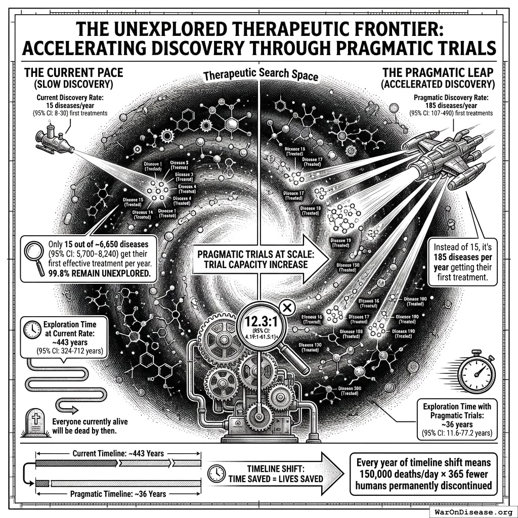
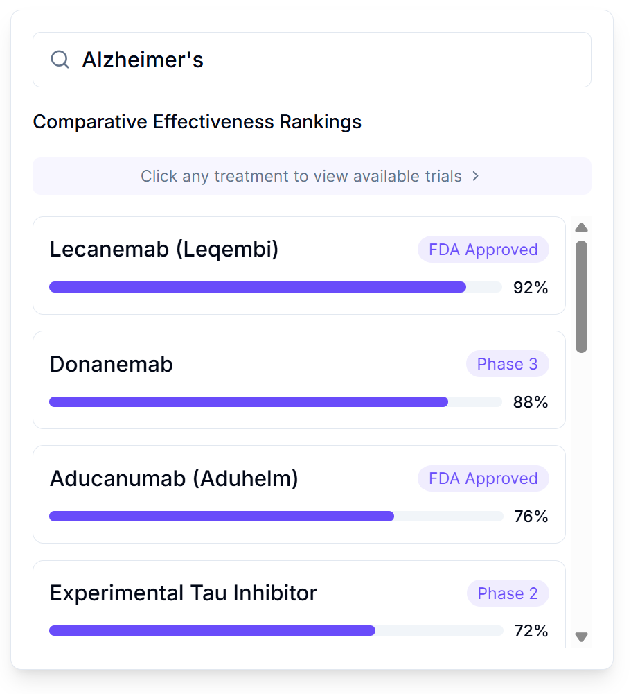
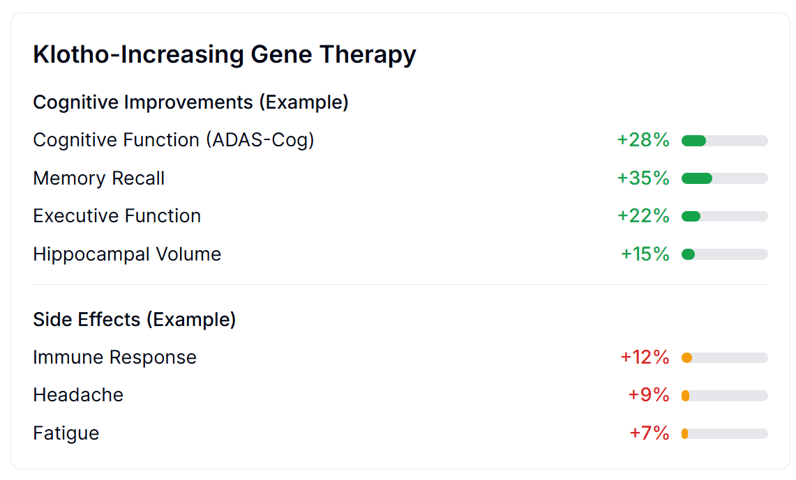
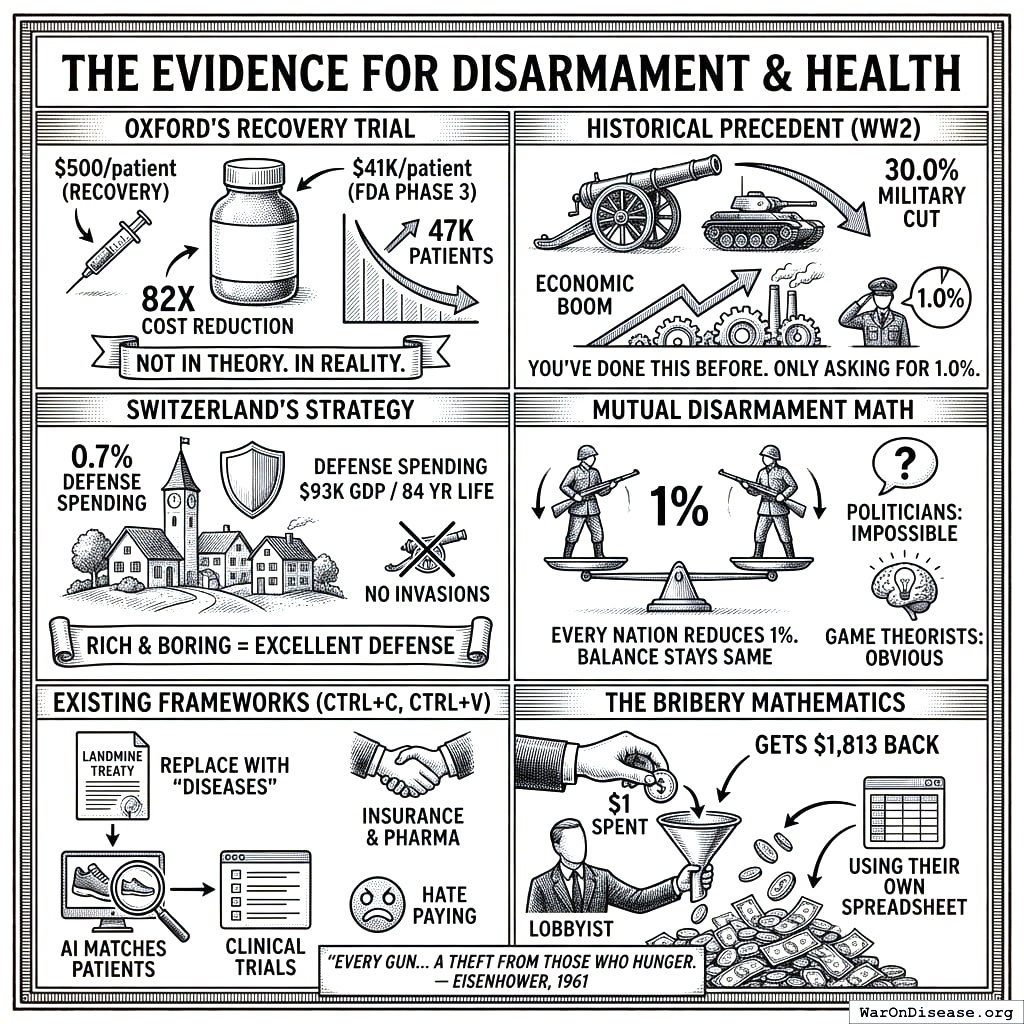
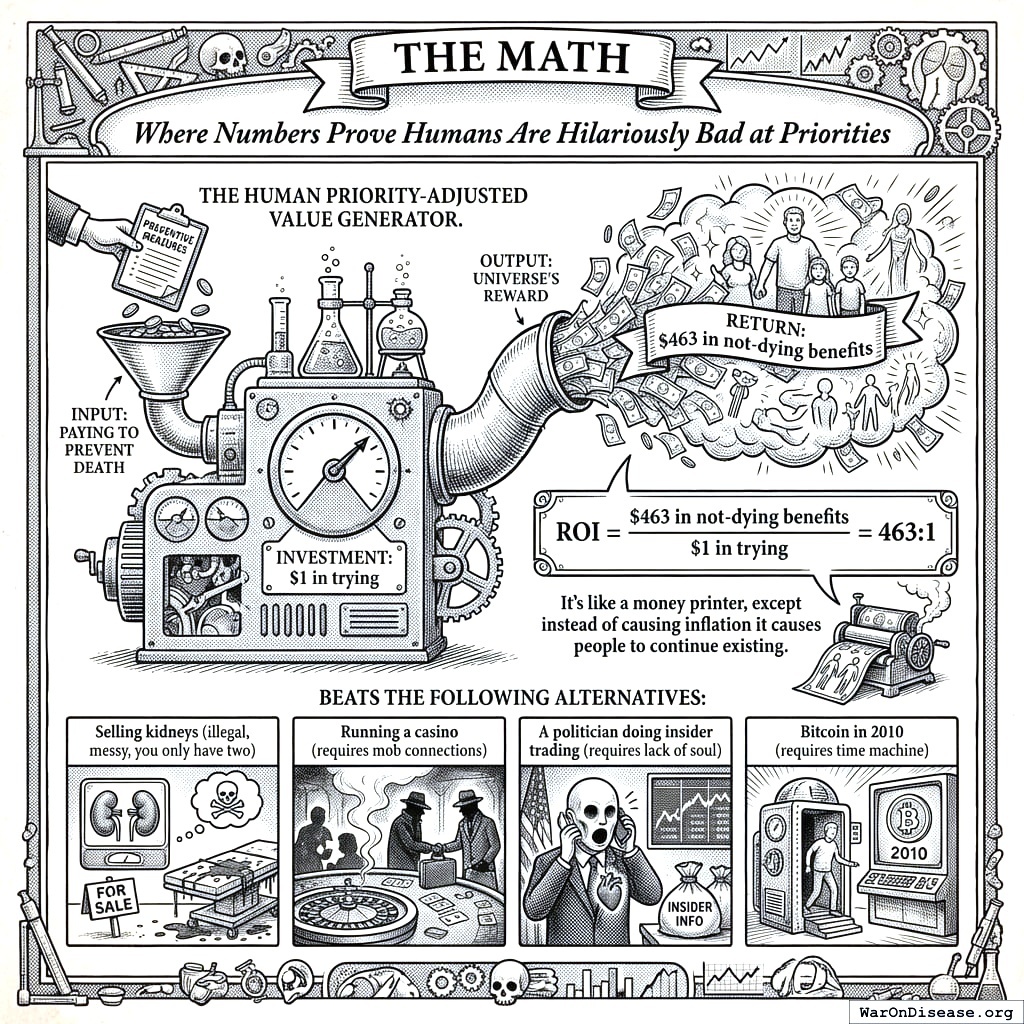
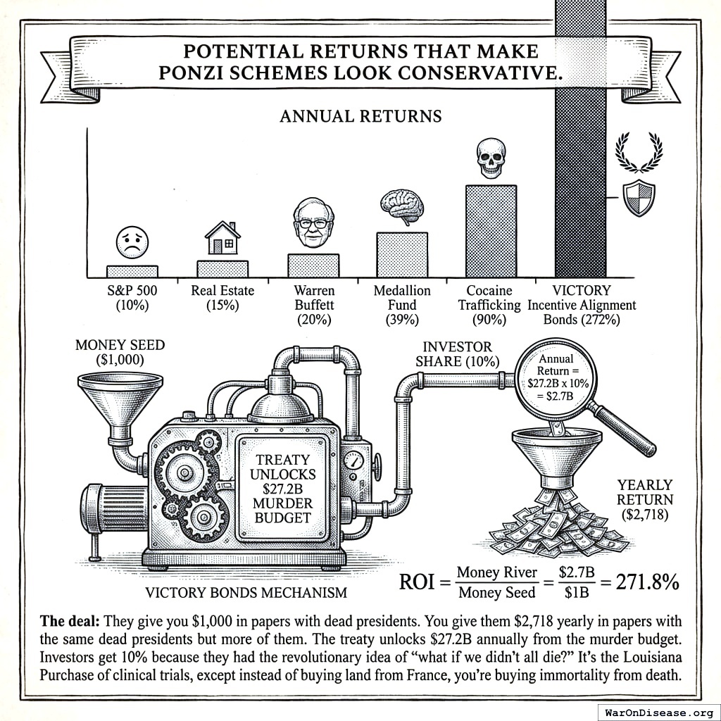
